Note
Go to the end to download the full example code.
Seeded uncertainty in methane generation#
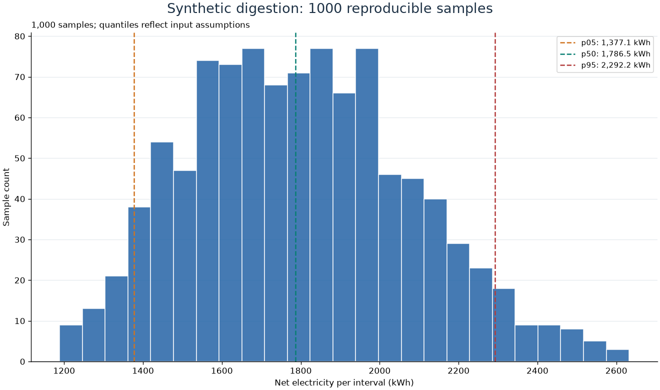
Independent uniform sampling illustrates how assumptions propagate to net electricity. These quantiles are not calibrated confidence intervals.
from x2power.utilities.experiments import monte_carlo
from x2power.utilities.plotting import plot_uncertainty
Methane yield is per kg volatile solids destroyed, not per kg volatile solids fed. The yield basis matters when destruction fraction is also uncertain.
scenario = {
    "schema_version": 1,
    "route": "digestion",
    "duration_h": 24,
    "feedstock": {"mass_kg": 10000, "moisture_fraction": 0.75, "dry_lhv_mj_per_kg": 18},
    "process": {
        "volatile_solids_fraction_dry": 0.9,
        "vs_destruction_fraction": 0.6,
        "methane_yield_nm3_per_kg_vs_destroyed": 0.5,
        "process_heat_kwh_per_kg_wet": 0.025,
    },
    "generator": {"electrical_efficiency": 0.35, "heat_recovery_efficiency": 0.4},
    "auxiliaries": {"fixed_power_kw": 3, "electricity_fraction_of_gross": 0.04},
}
samples = monte_carlo(
    scenario,
    {
        "process.vs_destruction_fraction": (0.45, 0.65),
        "process.methane_yield_nm3_per_kg_vs_destroyed": (0.4, 0.55),
        "generator.electrical_efficiency": (0.30, 0.38),
    },
    samples=1000,
    seed=42,
)
print(samples["net_electricity_kwh"])
{'p05': 1377.099311946574, 'p50': 1786.5299726545518, 'p95': 2292.2393090219452, 'mean': 1799.9674205309054}
Retained draws allow the reported distribution to be inspected and reproduced.
figure = plot_uncertainty(
    [draw["net_kwh"] for draw in samples["draws"]],
    title="Synthetic digestion: 1000 reproducible samples",
)
Total running time of the script: (0 minutes 0.144 seconds)