Note
Go to the end to download the full example code.
Tenerife banana residues: electricity and cost-benefit screening#
Use real published island context and laboratory substrate measurements to screen an assumed 5,000 wet-tonne/year pseudostem-to-electricity project. This is not an operating Tenerife plant or a supplier-quoted design. The substrate proxy was sampled in Gran Canaria, and the economic inputs are explicit assumptions.
Run this example from a repository checkout with pip install -e '.[plots]'.
The downloadable script and notebook use the accompanying analysis package
and its pinned input file; no live data service or credentials are required.
from analysis.tenerife_banana.case import load_case, sensitivities, simulate_case
from analysis.tenerife_banana.plots import (
    cash_flow_figure,
    cost_figure,
    energy_figure,
    operation_figure,
    sensitivity_figure,
)
1. Inspect provenance before running the model. The input file links every sourced observation to its publication and separates all engineering and cost assumptions. The 2024 fruit-production figure is context, not a feedstock supply estimate. Only raw pseudostem is modeled; fruit, leaves and rachis are excluded.
config = load_case()
context = config["region_context"]
measured = config["feedstock_measurements"]
print(
    f"Published Tenerife fruit-production context ({context['banana_fruit_production_year']}): "
    f"{context['banana_fruit_production_tonnes']:,.0f} tonnes"
)
print(f"Proxy sample location: {measured['sample_location']}")
print(f"Total solids: {measured['total_solids_fraction_wet']:.1%} of wet mass")
print(f"Volatile solids: {measured['volatile_solids_fraction_ts']:.1%} of total solids")
print(f"Laboratory BMP: {measured['methane_potential_nm3_per_kg_vs_fed']:.5f} Nm³/kg VS fed")
Published Tenerife fruit-production context (2024): 186,771 tonnes
Proxy sample location: Galdar, Gran Canaria; laboratory assays in Madrid
Total solids: 6.2% of wet mass
Volatile solids: 67.8% of total solids
Laboratory BMP: 0.36329 Nm³/kg VS fed
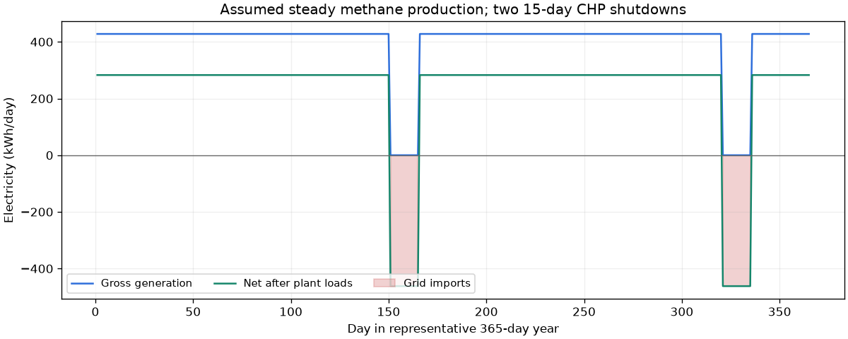
2. Apply a 70% BMP realization assumption before methane capture and generation. BMP is per VS fed, not VS destroyed. Laboratory yields do not establish continuous mono-digestion stability. Feed is uniform across a representative 365-day year; thirty CHP outage days still require plant electricity and heat. Recovered heat serves the digester; electric backup meets the remaining duty.
result = simulate_case(config)
metrics = result["metrics"]
print(f"Net electricity: {metrics['annual_net_electricity_kwh'] / 1000:.2f} MWh/year")
print(f"Positive deliveries: {metrics['annual_delivered_electricity_kwh'] / 1000:.2f} MWh/year")
print(f"Grid imports: {metrics['annual_imported_electricity_kwh'] / 1000:.2f} MWh/year")
energy = energy_figure(result)
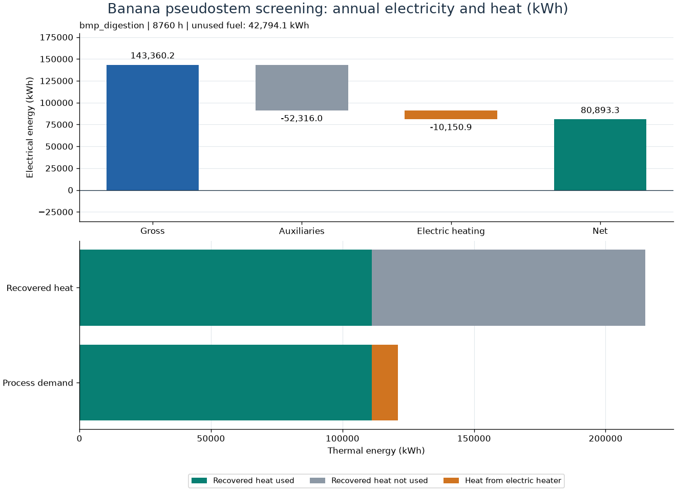
Net electricity: 80.89 MWh/year
Positive deliveries: 94.75 MWh/year
Grid imports: 13.86 MWh/year
3. See why annual netting would misprice the result. Exported energy is valued separately from the electricity purchased during shutdowns. There is no gas storage model: unused fuel remains reported, with no assumed emissions fate.
operation = operation_figure(result)
4. Account for collection, transport, labour, maintenance, residue handling and imported electricity. Baseline energy is sold at an assumed EUR 0.07/kWh; imports cost EUR 0.18/kWh. No gate fee, grant, avoided disposal charge, heat sale, digestate sale or carbon revenue is claimed. Costs are assumptions, not quotes.
costs = cost_figure(result)
print(f"Initial investment: EUR {sum(result['capital_costs_eur'].values()):,.0f}")
print(f"Annual operating balance: EUR {metrics['annual_operating_cash_flow_eur']:,.0f}")
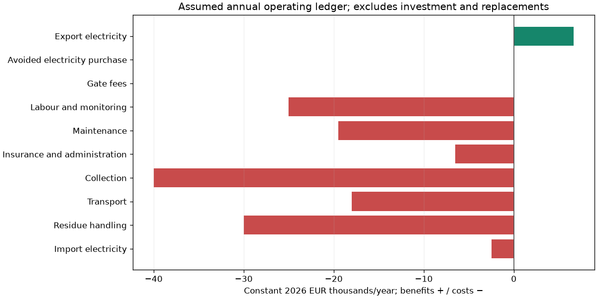
Initial investment: EUR 650,000
Annual operating balance: EUR -134,862
5. Discount 20 years of constant 2026-euro flows at 8% real. Include a year-10 replacement and year-20 decommissioning. This is unlevered and pre-tax. Gross LCOE includes all stated costs and plant import purchases; its denominator is positive electricity delivered after plant loads, not gross CHP generation.
finance = result["cost_benefit"]
print(f"NPV: EUR {finance['net_present_value']:,.0f}")
print(f"Benefit/cost ratio: {finance['benefit_cost_ratio']:.3f}")
print(f"Gross LCOE: EUR {finance['levelized_cost_per_kwh']:.3f}/kWh")
print(f"Simple payback within horizon: {finance['simple_payback_years']}")
cash_flow = cash_flow_figure(result)
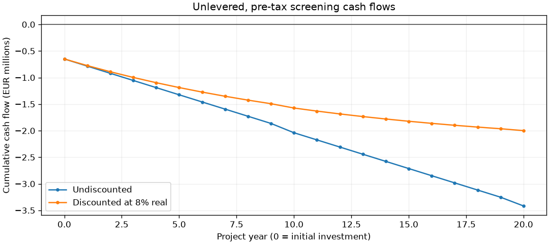
NPV: EUR -1,999,062
Benefit/cost ratio: 0.032
Gross LCOE: EUR 2.219/kWh
Simple payback within horizon: None
6. Test a hypothetical gate fee and the value of delivered electricity while holding other inputs, including import price, fixed. The zero contour is an arithmetic threshold, not an available contract. A fee must come from an actual payer; do not also count the same avoided disposal cost. Yield stress tests are deterministic assumptions, not statistical confidence intervals.
stress_tests = sensitivities(config, result)
sensitivity = sensitivity_figure(stress_tests)
print(f"Break-even total gate fee: EUR {metrics['break_even_total_gate_fee_eur_per_tonne']:.2f}/t")
for row in stress_tests["bmp_realization"]:
    print(
        f"BMP realization {row['bmp_realization_fraction']:.0%}: "
        f"net {row['net_electricity_kwh'] / 1000:.2f} MWh/year; "
        f"NPV EUR {row['net_present_value_eur']:,.0f}"
    )
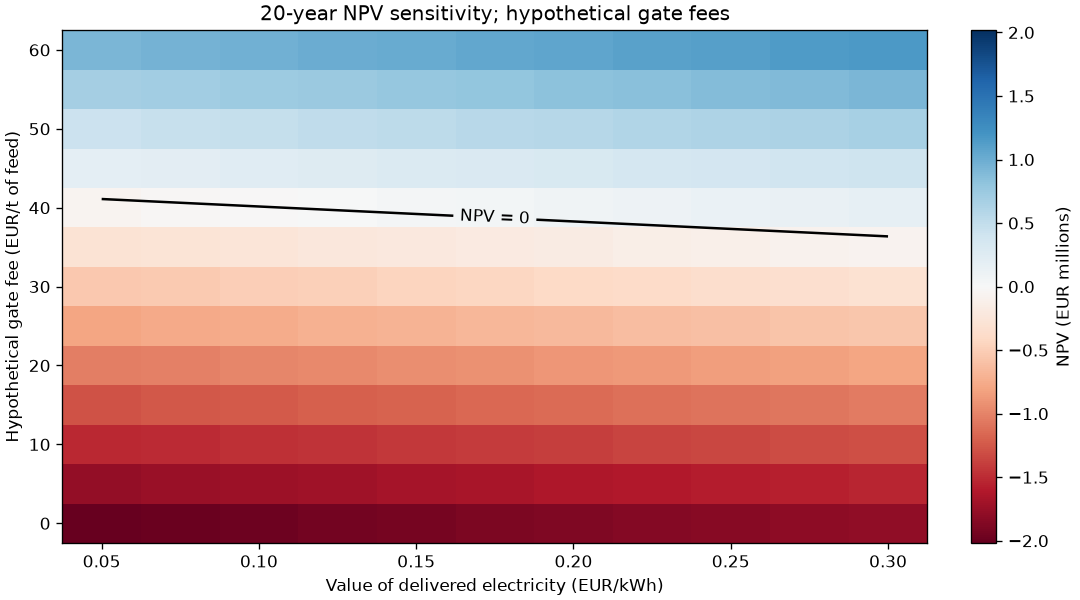
Break-even total gate fee: EUR 40.72/t
BMP realization 50%: net 41.98 MWh/year; NPV EUR -2,025,805
BMP realization 70%: net 80.89 MWh/year; NPV EUR -1,999,062
BMP realization 90%: net 119.81 MWh/year; NPV EUR -1,972,319
The baseline is financially negative under these assumptions. Before changing that conclusion, measure local feed TS/VS/BMP and seasonal supply, demonstrate stable digestion, obtain equipment/haulage quotes and establish a credible energy user or buyer. Co-digestion and shared infrastructure need a separate model.
Reproduce all JSON/CSV and PNG/SVG results with:
python -m analysis.tenerife_banana.run --plot.
See Tenerife banana residues: electricity feasibility case for source locators, equations and exclusions.
Total running time of the script: (0 minutes 0.493 seconds)