Note
Go to the end to download the full example code.
Compact orbital compute clusters and distributed power#
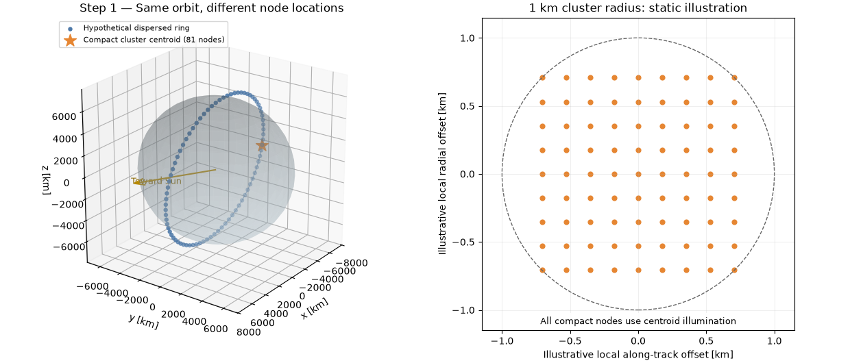
Explore how constellation geometry changes the timing of solar generation. Google’s Suncatcher paper illustrates a proposed 81-satellite cluster at 650 km altitude, within a 1 km radius, for a future dawn-dusk sun-synchronous architecture. This example uses that count and altitude as a design scenario. It compares a compact cluster with an explicitly hypothetical 81-node ring spread evenly around the same orbital plane.
The compact cluster uses its centroid’s illumination for all 81 nodes. The local square layout is a static illustration, not a propagation of Google’s formation or a collision-avoidance solution. A kilometre-scale cluster has strongly correlated Earth eclipses; small differences at shadow boundaries are omitted by the centroid approximation. The distributed ring is a separate comparison, not the published Suncatcher architecture.
Source and status#
Google, Towards a future space-based, highly scalable AI infrastructure system design, Section 2.2 and Figure 2: https://services.google.com/fh/files/misc/suncatcher_paper.pdf
Google announced a single hardware prototype in orbit on October 1, 2026: https://blog.google/innovation-and-ai/models-and-research/google-research/project-suncatcher-prototype/
That prototype does not establish an operational 81-satellite data center. All electrical ratings below are declared modelling assumptions, and the outputs are simulated rather than measured mission generation.
Model assumptions#
Use a circular 650 km orbit, first-order J2 sun-synchronous inclination, 06:00 mean local time of the ascending node, and an idealized northern winter solstice. The Sun remains fixed over the one-orbit comparison, at 1 AU. Earth is spherical, and the finite solar disc gives gradual eclipse edges. Each node has an assumed 100 kW DC reference array at 1361 W/m² and 25°C, held normal to the Sun at fixed temperature, and an assumed constant 60 kW electrical load. Array shading by other spacecraft, degradation, thermal response, electrical losses, storage, and power transfer are not modelled.
import matplotlib.pyplot as plt
import numpy as np
from matplotlib.patches import Circle

import orbitalpv as opv
At the idealized winter solstice the ecliptic longitude is 270 degrees. A constant mean nodal rate tracks that longitude. The local-time helper therefore receives the mean Sun angle, rather than an apparent right ascension that would introduce the equation of time into this convention.
nodes = 81
altitude_m = 650_000.0
cluster_radius_km = 1.0
inclination_deg = opv.sun_synchronous_inclination_deg(altitude_m)
period_s = opv.circular_orbit_period_s(altitude_m)
obliquity_rad = np.deg2rad(23.43928)
solar_longitude_rad = 3.0 * np.pi / 2.0
sun_unit = np.array(
    [
        np.cos(solar_longitude_rad),
        np.cos(obliquity_rad) * np.sin(solar_longitude_rad),
        np.sin(obliquity_rad) * np.sin(solar_longitude_rad),
    ]
)
sun_position_m = opv.ASTRONOMICAL_UNIT_M * sun_unit
raan_deg = opv.raan_from_local_solar_time_deg(
    6.0, sun_right_ascension_deg=np.rad2deg(solar_longitude_rad)
)
orbit_radius_m = opv.EARTH_EQUATORIAL_RADIUS_M + altitude_m

# An integer number of samples between neighboring ring nodes makes their
# phase shifts exact on this time grid. The repeated endpoint closes the orbit
# for integrations; it is excluded from the illumination heatmaps.
samples_per_node = 40
sample_count = nodes * samples_per_node
phase_rad = np.linspace(0.0, 2.0 * np.pi, sample_count, endpoint=False)
positions_m = opv.keplerian_orbit_positions_m(
    orbit_radius_m,
    0.0,
    inclination_deg,
    raan_deg=raan_deg,
    true_anomaly_rad=phase_rad,
)
time_s = np.linspace(0.0, period_s, sample_count + 1)
time_min = time_s / 60.0
ring_positions_km = positions_m[::samples_per_node] / 1000.0
orbit_km = np.vstack([positions_m, positions_m[:1]]) / 1000.0

fig = plt.figure(figsize=(12.4, 5.3), layout="constrained")
ax = fig.add_subplot(1, 2, 1, projection="3d")
longitude, latitude = np.meshgrid(np.linspace(0, 2 * np.pi, 41), np.linspace(0, np.pi, 21))
earth_radius_km = opv.EARTH_EQUATORIAL_RADIUS_M / 1000.0
ax.plot_surface(
    earth_radius_km * np.cos(longitude) * np.sin(latitude),
    earth_radius_km * np.sin(longitude) * np.sin(latitude),
    earth_radius_km * np.cos(latitude),
    color="#BCCED8",
    alpha=0.28,
    linewidth=0,
)
ax.plot(*orbit_km.T, color="#4C78A8", linewidth=0.8, alpha=0.6)
ax.scatter(*ring_positions_km.T, s=13, color="#4C78A8", label="Hypothetical dispersed ring")
ax.scatter(
    *ring_positions_km[0],
    marker="*",
    s=180,
    color="#E68632",
    label="Compact cluster centroid (81 nodes)",
    depthshade=False,
)
ax.quiver(0, 0, 0, *sun_unit, length=9_000, color="#B88900", arrow_length_ratio=0.13)
ax.text(*(9_400 * sun_unit), "Toward Sun", color="#8B6800", fontsize=9)
ax.set(
    xlabel="x [km]",
    ylabel="y [km]",
    zlabel="z [km]",
    title="Step 1 — Same orbit, different node locations",
)
ax.set_box_aspect((1, 1, 1))
ax.view_init(elev=23, azim=36)
ax.legend(loc="upper left", fontsize=8)

ax = fig.add_subplot(1, 2, 2)
coordinate_km = np.linspace(-1.0, 1.0, 9) * cluster_radius_km / np.sqrt(2.0)
along_track_km, radial_km = np.meshgrid(coordinate_km, coordinate_km)
ax.scatter(along_track_km.ravel(), radial_km.ravel(), s=24, color="#E68632")
ax.add_patch(Circle((0, 0), cluster_radius_km, fill=False, linestyle="--", color="#666666"))
ax.set(
    xlabel="Illustrative local along-track offset [km]",
    ylabel="Illustrative local radial offset [km]",
    title="1 km cluster radius: static illustration",
    xlim=(-1.15, 1.15),
    ylim=(-1.15, 1.15),
    aspect="equal",
)
ax.text(
    0.5,
    0.02,
    "All compact nodes use centroid illumination",
    transform=ax.transAxes,
    ha="center",
    fontsize=9,
    bbox={"facecolor": "white", "edgecolor": "none", "alpha": 0.9},
)
ax.grid(alpha=0.2)
plt.show()
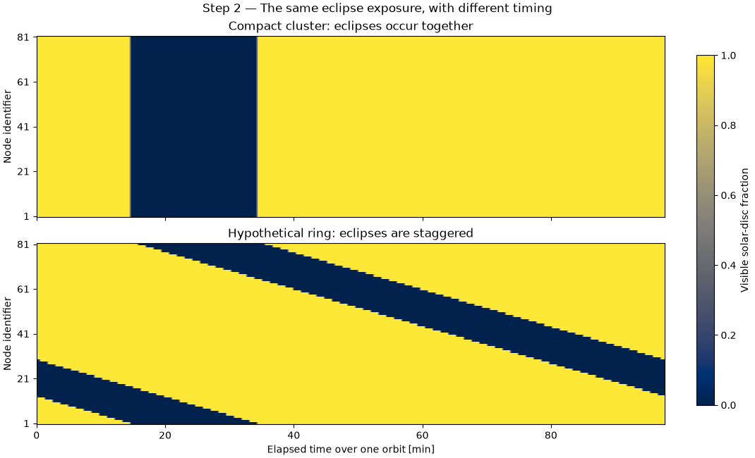
earth_occultation_fraction returns the visible fraction of the solar
disc: one is fully illuminated, zero is full Earth shadow. A phase shift of
the same closed orbit is sufficient here because the Sun is frozen over one
revolution. It is not a long-term formation-flight propagator.
centroid_illumination = np.array(
    [opv.earth_occultation_fraction(position, sun_position_m) for position in positions_m]
)
compact_illumination = np.broadcast_to(centroid_illumination, (nodes, sample_count))
shifted_indices = (
    np.arange(nodes)[:, None] * samples_per_node + np.arange(sample_count)[None, :]
) % sample_count
ring_illumination = centroid_illumination[shifted_indices]

fig, axes = plt.subplots(2, 1, figsize=(10.7, 6.5), sharex=True, layout="constrained")
for ax, illumination, title in zip(
    axes,
    (compact_illumination, ring_illumination),
    ("Compact cluster: eclipses occur together", "Hypothetical ring: eclipses are staggered"),
    strict=True,
):
    plotted = ax.imshow(
        illumination,
        origin="lower",
        aspect="auto",
        interpolation="nearest",
        extent=(0, period_s / 60.0, 0.5, nodes + 0.5),
        vmin=0.0,
        vmax=1.0,
        cmap="cividis",
    )
    ax.set(ylabel="Node identifier", title=title, yticks=[1, 21, 41, 61, 81])
axes[-1].set_xlabel("Elapsed time over one orbit [min]")
fig.colorbar(plotted, ax=axes, label="Visible solar-disc fraction", shrink=0.9)
fig.suptitle("Step 2 — The same eclipse exposure, with different timing")
plt.show()
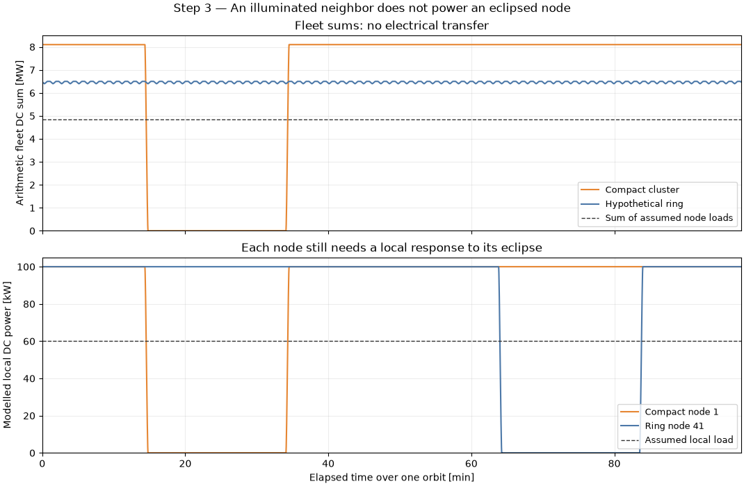
A smooth arithmetic sum across a distributed fleet does not supply a node that is inside Earth’s shadow. Compute each node’s DC output independently. The 100 kW array and 60 kW load are illustrative choices, not Google hardware specifications. The ring’s node 41 is chosen to make its shifted eclipse visible; all nodes have the same one-orbit exposure in this frozen geometry.
reference = opv.PvwattsReference(
    pdc0_w=100_000.0,
    gamma_pdc_per_c=-0.003,
    reference_irradiance_w_m2=1361.0,
    reference_temperature_c=25.0,
)
load_per_node_w = 60_000.0
compact_closed = np.column_stack([compact_illumination, compact_illumination[:, 0]])
ring_closed = np.column_stack([ring_illumination, ring_illumination[:, 0]])
compact_dc_w = opv.pvwatts_dc_space(1361.0 * compact_closed, 25.0, reference)
ring_dc_w = opv.pvwatts_dc_space(1361.0 * ring_closed, 25.0, reference)
compact_fleet_w = compact_dc_w.sum(axis=0)
ring_fleet_w = ring_dc_w.sum(axis=0)

fig, axes = plt.subplots(2, 1, figsize=(10.7, 7), sharex=True, layout="constrained")
axes[0].plot(time_min, compact_fleet_w / 1e6, color="#E68632", label="Compact cluster")
axes[0].plot(time_min, ring_fleet_w / 1e6, color="#4C78A8", label="Hypothetical ring")
axes[0].axhline(
    nodes * load_per_node_w / 1e6,
    color="#333333",
    linestyle="--",
    linewidth=1,
    label="Sum of assumed node loads",
)
axes[0].set(ylabel="Arithmetic fleet DC sum [MW]", title="Fleet sums: no electrical transfer")
axes[0].legend(fontsize=9, loc="lower right")
axes[1].plot(time_min, compact_dc_w[0] / 1000, color="#E68632", label="Compact node 1")
axes[1].plot(time_min, ring_dc_w[40] / 1000, color="#4C78A8", label="Ring node 41")
axes[1].axhline(
    load_per_node_w / 1000,
    color="#333333",
    linestyle="--",
    linewidth=1,
    label="Assumed local load",
)
axes[1].set(
    xlabel="Elapsed time over one orbit [min]",
    ylabel="Modelled local DC power [kW]",
    title="Each node still needs a local response to its eclipse",
)
axes[1].legend(fontsize=9, loc="lower right")
for ax in axes:
    ax.set_xlim(0, period_s / 60.0)
    ax.set_ylim(bottom=0)
    ax.grid(alpha=0.22)
fig.suptitle("Step 3 — An illuminated neighbor does not power an eclipsed node")
plt.show()
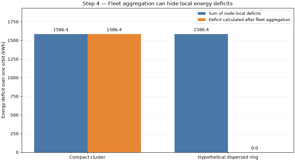
Integrate max(local load - local generation, 0) for every node before taking the sum. Reversing these operations hides the ring’s local deficits because generation elsewhere offsets them arithmetically. These are energy shortfalls without storage or load shifting, not battery nameplate ratings; a storage design also needs efficiency, usable capacity, and power limits.
local_deficit_kwh = []
aggregate_deficit_kwh = []
for node_power_w in (compact_dc_w, ring_dc_w):
    per_node_kwh = (
        np.trapezoid(np.maximum(load_per_node_w - node_power_w, 0.0), time_s, axis=1) / 3_600_000.0
    )
    local_deficit_kwh.append(float(per_node_kwh.sum()))
    aggregate_deficit_kwh.append(
        float(
            np.trapezoid(
                np.maximum(nodes * load_per_node_w - node_power_w.sum(axis=0), 0.0), time_s
            )
            / 3_600_000.0
        )
    )

fig, ax = plt.subplots(figsize=(9.5, 5.2), layout="constrained")
architecture = np.arange(2)
bars_local = ax.bar(
    architecture - 0.19,
    local_deficit_kwh,
    0.38,
    color="#4C78A8",
    label="Sum of node-local deficits",
)
bars_aggregate = ax.bar(
    architecture + 0.19,
    aggregate_deficit_kwh,
    0.38,
    color="#E68632",
    label="Deficit calculated after fleet aggregation",
)
ax.bar_label(bars_local, fmt="%.1f", padding=4)
ax.bar_label(bars_aggregate, fmt="%.1f", padding=4)
ax.set(
    xticks=architecture,
    xticklabels=["Compact cluster", "Hypothetical dispersed ring"],
    ylabel="Energy deficit over one orbit [kWh]",
    title="Step 4 — Fleet aggregation can hide local energy deficits",
    ylim=(0, max(local_deficit_kwh) * 1.22),
)
ax.grid(axis="y", alpha=0.22)
ax.set_axisbelow(True)
ax.legend(loc="upper right", fontsize=9)
plt.show()

print(f"Concept scenario: {nodes} nodes, {altitude_m / 1000:.0f} km, 06:00 mean LTAN")
print(f"J2 inclination: {inclination_deg:.6f} deg; period: {period_s / 60:.6f} min")
print(f"Time spacing: {period_s / sample_count:.3f} s; finite solar disc at 1 AU")
print(f"Modelled sunlight-equivalent fraction: {centroid_illumination.mean():.6f}")
print("Assumed per-node reference array: 100 kW DC; assumed continuous load: 60 kW")
for name, local, aggregate in zip(
    ("Compact cluster", "Hypothetical ring"),
    local_deficit_kwh,
    aggregate_deficit_kwh,
    strict=True,
):
    print(
        f"{name}: mean local deficit {local / nodes:.3f} kWh/node/orbit; "
        f"sum of local deficits {local:.3f} kWh; "
        f"deficit after fleet aggregation {aggregate:.3f} kWh"
    )
Concept scenario: 81 nodes, 650 km, 06:00 mean LTAN
J2 inclination: 97.985997 deg; period: 97.728236 min
Time spacing: 1.810 s; finite solar disc at 1 AU
Modelled sunlight-equivalent fraction: 0.798120
Assumed per-node reference array: 100 kW DC; assumed continuous load: 60 kW
Compact cluster: mean local deficit 19.585 kWh/node/orbit; sum of local deficits 1586.367 kWh; deficit after fleet aggregation 1586.367 kWh
Hypothetical ring: mean local deficit 19.585 kWh/node/orbit; sum of local deficits 1586.367 kWh; deficit after fleet aggregation 0.000 kWh
Total running time of the script: (0 minutes 0.966 seconds)