Note
Go to the end to download the full example code.
Sentinel-2 polar imaging and solar-power geometry#
Explore the nominal Sentinel-2B/2C pair through OrbitalPV’s public API: its orbital plane, Earth-fixed subpoint tracks, daylight below each spacecraft, and an illustrative onboard photovoltaic power profile.
Mission parameters and scope#
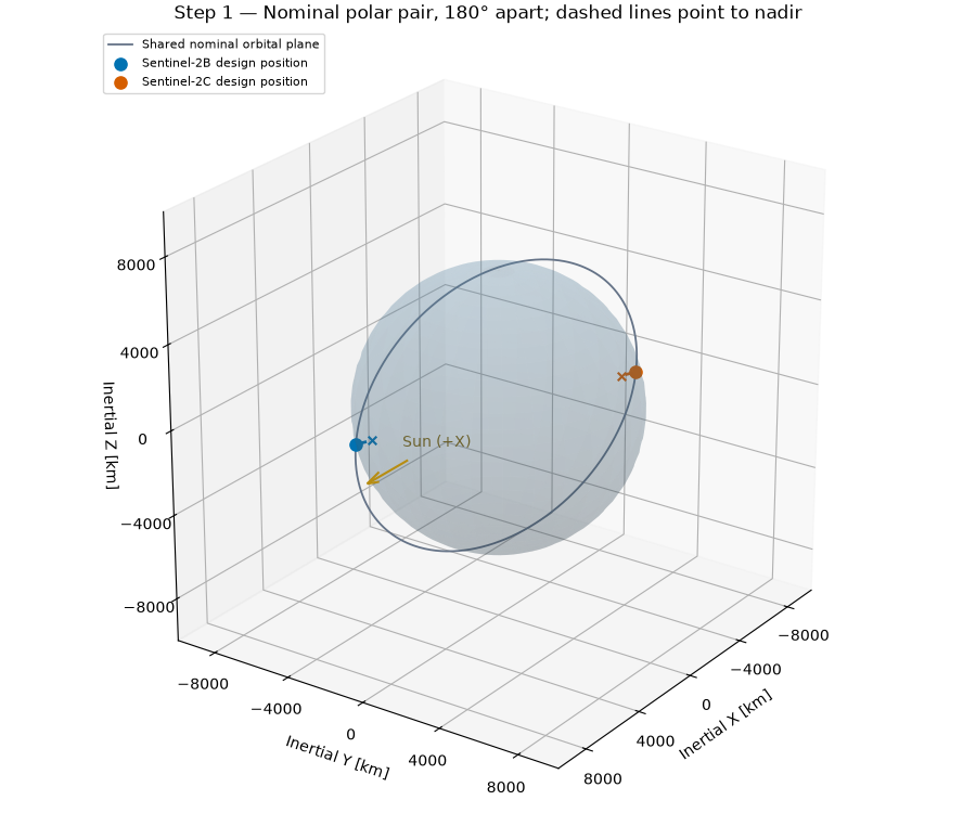
The Copernicus mission description specifies a mean altitude of 786 km, inclination 98.62 degrees, and 10:30 mean local solar time at the descending node. The nominal pair occupies the same orbit, 180 degrees apart. We model that pair; the separate Sentinel-2A extension campaign is outside this example.
Sources:
Mission orbit and constellation: https://sentiwiki.copernicus.eu/web/s2-mission
Imaging products: https://sentiwiki.copernicus.eu/web/s2-products
ESA constellation overview: https://www.esa.int/Applications/Observing_the_Earth/Copernicus/Sentinel-2/Satellite_constellation
Sentinel-2’s MSI measures reflected sunlight. Its imagery and surface reflectance can provide land-surface context for energy studies; this example does not retrieve or calculate ground irradiance. Solar radiation mapping also needs suitable atmospheric and cloud information and a validated radiative-transfer method.
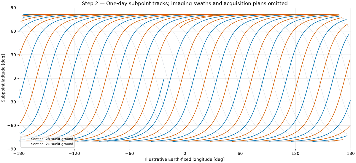
The model uses a circular two-body orbit, spherical rotating Earth and a fixed Sun along the inertial +X axis at an idealized equinox. Time zero is a designed descending-node crossing for B, with Greenwich angle zero. There is no real acquisition epoch or operational ephemeris. The calculation does not propagate the nodal precession that maintains a real sun-synchronous orbit, nor reproduce the mission’s repeat cycle, swath, cloud cover or acquisition plan. The map shows subpoints, not an image-coverage or revisit forecast.
PV assumptions are separate from the mission facts: each spacecraft is assigned an illustrative 1 kW AM0 reference array, ideal Sun tracking, 40 °C cell temperature and a 0.95 optical factor. These are not Sentinel-2 hardware specifications. Batteries, loads and thermal dynamics are not modeled.
from __future__ import annotations

import matplotlib.pyplot as plt
import numpy as np

import orbitalpv as opv
The descending-node local time sets the orbital-plane orientation relative to the chosen Sun direction. The helper accounts for the 12-hour difference between ascending and descending crossings. The initial phases below are designed, while the 180-degree separation follows the mission specification.
ALTITUDE_M = 786_000.0
INCLINATION_DEG = 98.62
DESCENDING_LOCAL_TIME_H = 10.5
SPACECRAFT = ("Sentinel-2B design position", "Sentinel-2C design position")
COLORS = ("#0072B2", "#D55E00")
PHASE_DEG = (180.0, 360.0)

earth_radius_m = opv.EARTH_EQUATORIAL_RADIUS_M
orbit_radius_m = earth_radius_m + ALTITUDE_M
period_s = opv.circular_orbit_period_s(ALTITUDE_M)
raan_deg = opv.raan_from_local_solar_time_deg(
    DESCENDING_LOCAL_TIME_H,
    sun_right_ascension_deg=0.0,
    ascending=False,
)
time_s = np.arange(0.0, 86_400.0 + 30.0, 30.0)
sun_position_m = np.array([opv.ASTRONOMICAL_UNIT_M, 0.0, 0.0])
positions = {}
illumination = {}
daylight_cosine = {}
sun_distance_m = {}
tracks = {}

for spacecraft, phase_deg in zip(SPACECRAFT, PHASE_DEG, strict=True):
    anomaly = np.deg2rad(phase_deg) + 2.0 * np.pi * time_s / period_s
    position = opv.keplerian_orbit_positions_m(
        orbit_radius_m,
        eccentricity=0.0,
        inclination_deg=INCLINATION_DEG,
        raan_deg=raan_deg,
        true_anomaly_rad=anomaly,
    )
    geometry = [opv.solar_geometry(point, sun_position_m) for point in position]
    positions[spacecraft] = position
    illumination[spacecraft] = np.array([item.illumination_fraction for item in geometry])
    sun_distance_m[spacecraft] = np.array([item.sun_distance_m for item in geometry])
    subpoints = earth_radius_m * position / np.linalg.norm(position, axis=1)[:, None]
    daylight_cosine[spacecraft] = np.array(
        [opv.cosine_incidence(point, sun_position_m - point) for point in subpoints]
    )
    tracks[spacecraft] = opv.ground_track_deg_from_eci(position, time_s)

print(f"Nominal altitude: {ALTITUDE_M / 1000:.0f} km; inclination: {INCLINATION_DEG:.2f} deg")
print(f"Two-body circular period: {period_s / 60.0:.2f} min")
print(f"10:30 descending local time gives RAAN {raan_deg:.1f} deg for the assumed Sun")
print("Epoch and Greenwich angle are illustrative; no live satellite elements are used.")

orbit_curve_km = (
    opv.circular_orbit_positions_m(ALTITUDE_M, INCLINATION_DEG, raan_deg=raan_deg) / 1000.0
)
earth_radius_km = earth_radius_m / 1000.0
longitude = np.linspace(0.0, 2.0 * np.pi, 60)
colatitude = np.linspace(0.0, np.pi, 30)
earth_x = earth_radius_km * np.outer(np.cos(longitude), np.sin(colatitude))
earth_y = earth_radius_km * np.outer(np.sin(longitude), np.sin(colatitude))
earth_z = earth_radius_km * np.outer(np.ones_like(longitude), np.cos(colatitude))

fig = plt.figure(figsize=(9, 7.5), layout="constrained")
ax = fig.add_subplot(111, projection="3d")
ax.plot_surface(earth_x, earth_y, earth_z, color="#6699bb", alpha=0.18, linewidth=0)
ax.plot(*orbit_curve_km.T, color="#657387", linewidth=1.3, label="Shared nominal orbital plane")
for spacecraft, color in zip(SPACECRAFT, COLORS, strict=True):
    point_km = positions[spacecraft][0] / 1000.0
    subpoint_km = earth_radius_km * point_km / np.linalg.norm(point_km)
    ax.scatter(*point_km, color=color, s=65, label=spacecraft)
    ax.plot(
        *np.vstack([point_km, subpoint_km]).T,
        color=color,
        linewidth=2.0,
        linestyle="--",
    )
    ax.scatter(*subpoint_km, color=color, marker="x", s=30)
ax.quiver(1.04 * earth_radius_km, 0, 0, 0.45 * earth_radius_km, 0, 0, color="#b78d12")
ax.text(1.1 * earth_radius_km, 0, 0.12 * earth_radius_km, "Sun (+X)", color="#84660e")
limit_km = 1.4 * orbit_radius_m / 1000.0
ax.set(xlim=(-limit_km, limit_km), ylim=(-limit_km, limit_km), zlim=(-limit_km, limit_km))
ax.set(xlabel="Inertial X [km]", ylabel="Inertial Y [km]", zlabel="Inertial Z [km]")
ticks_km = np.arange(-8000, 8001, 4000)
ax.set(xticks=ticks_km, yticks=ticks_km, zticks=ticks_km)
ax.set_box_aspect((1, 1, 1))
ax.view_init(elev=24, azim=35)
ax.set_title("Step 1 — Nominal polar pair, 180° apart; dashed lines point to nadir")
ax.legend(loc="upper left", fontsize=8)
plt.show()
Nominal altitude: 786 km; inclination: 98.62 deg
Two-body circular period: 100.58 min
10:30 descending local time gives RAAN 157.5 deg for the assumed Sun
Epoch and Greenwich angle are illustrative; no live satellite elements are used.
Grey trajectories show both day and night passes. Colored trajectories mark sunlit ground below each spacecraft. Latitude/longitude use the public spherical-Earth transform, with an arbitrary longitude origin at time zero. No sensor swath is applied, and daylight alone does not imply an acquisition.
fig, ax = plt.subplots(figsize=(12, 5.5), layout="constrained")
for spacecraft, color in zip(SPACECRAFT, COLORS, strict=True):
    lon_deg, lat_deg = tracks[spacecraft]
    wrapped_lon = lon_deg.copy()
    wrapped_lat = lat_deg.copy()
    dateline_jumps = np.flatnonzero(np.abs(np.diff(lon_deg)) > 180.0) + 1
    wrapped_lon[dateline_jumps] = np.nan
    wrapped_lat[dateline_jumps] = np.nan
    ax.plot(wrapped_lon, wrapped_lat, color="#a9b1ba", linewidth=0.6, alpha=0.5)
    night = daylight_cosine[spacecraft] <= 0.0
    lit_lon, lit_lat = wrapped_lon.copy(), wrapped_lat.copy()
    lit_lon[night], lit_lat[night] = np.nan, np.nan
    ax.plot(
        lit_lon,
        lit_lat,
        color=color,
        linewidth=1.2,
        label=spacecraft.replace(" design position", "") + " sunlit ground",
    )
ax.set(
    xlim=(-180, 180),
    ylim=(-90, 90),
    xlabel="Illustrative Earth-fixed longitude [deg]",
    ylabel="Subpoint latitude [deg]",
    title="Step 2 — One-day subpoint tracks; imaging swaths and acquisition plans omitted",
)
ax.set_xticks(np.arange(-180, 181, 60))
ax.set_yticks(np.arange(-90, 91, 30))
ax.grid(alpha=0.25)
ax.legend(loc="lower left", fontsize=8)
plt.show()
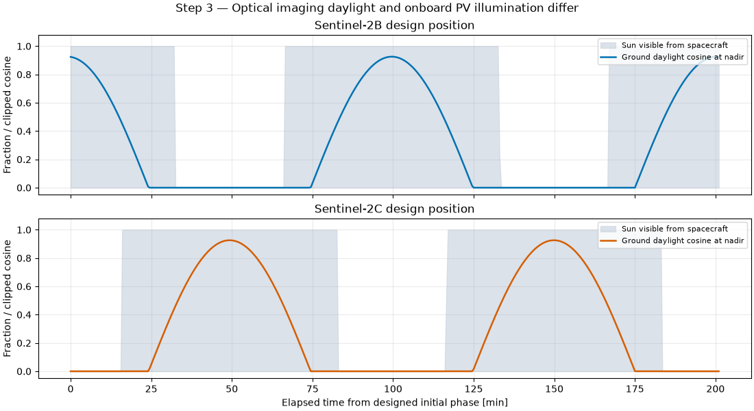
A spacecraft may still see the Sun while looking at a dark nadir point. The solid curve is the clipped cosine of the ground solar zenith angle, computed with the outward surface normal. The shaded curve is the fraction of the solar disc visible from the spacecraft. These are different geometric quantities, even though both range from zero to one.
shown = time_s <= 2.0 * period_s
elapsed_min = time_s[shown] / 60.0
fig, axes = plt.subplots(2, 1, figsize=(11, 6), sharex=True, layout="constrained")
for ax, spacecraft, color in zip(axes, SPACECRAFT, COLORS, strict=True):
    ax.fill_between(
        elapsed_min,
        0,
        illumination[spacecraft][shown],
        color="#c9d3df",
        alpha=0.65,
        label="Sun visible from spacecraft",
    )
    ax.plot(
        elapsed_min,
        daylight_cosine[spacecraft][shown],
        color=color,
        linewidth=1.8,
        label="Ground daylight cosine at nadir",
    )
    ax.set(title=spacecraft, ylabel="Fraction / clipped cosine", ylim=(-0.05, 1.08))
    ax.grid(alpha=0.25)
    ax.legend(loc="upper right", fontsize=8)
axes[-1].set_xlabel("Elapsed time from designed initial phase [min]")
fig.suptitle("Step 3 — Optical imaging daylight and onboard PV illumination differ")
plt.show()
Both spacecraft use the same explicitly assumed array model. Ideal Sun tracking gives unit incidence cosine while the array is illuminated. OrbitalPV supplies Sun distance, eclipse fraction, AM0 irradiance and the PVWatts calculation. The resulting profiles are simulated design quantities, not measured Sentinel-2 electrical output. The 24-hour summary spans a noninteger number of orbits, so the phase offset gives the identical array designs slightly different window-integrated energy.
reference = opv.PvwattsReference(
    pdc0_w=1000.0,
    gamma_pdc_per_c=-0.002,
    reference_irradiance_w_m2=1361.0,
    reference_temperature_c=25.0,
)
power_w = {}
for spacecraft in SPACECRAFT:
    incident = opv.am0_irradiance(sun_distance_m[spacecraft])
    effective = opv.effective_irradiance_w_m2(
        incident, illumination[spacecraft], np.ones_like(time_s), optical_factor=0.95
    )
    power_w[spacecraft] = opv.pvwatts_dc_space(effective, 40.0, reference)
    energy_kwh = float(np.trapezoid(power_w[spacecraft], time_s) / 3.6e6)
    sun_visible_fraction = float(np.trapezoid(illumination[spacecraft], time_s) / time_s[-1])
    print(
        f"{spacecraft}: illustrative 24 h DC energy {energy_kwh:.2f} kWh; mean Sun visibility {sun_visible_fraction:.1%}"
    )

fleet_power_w = np.sum(np.stack(list(power_w.values())), axis=0)
fig, axes = plt.subplots(2, 1, figsize=(11, 6), sharex=True, layout="constrained")
for spacecraft, color in zip(SPACECRAFT, COLORS, strict=True):
    axes[0].plot(
        elapsed_min,
        power_w[spacecraft][shown] / 1000.0,
        color=color,
        label=spacecraft.replace(" design position", ""),
    )
axes[0].set(
    ylabel="Illustrative DC power [kW]", title="Per spacecraft: assumed 1 kW AM0 reference array"
)
axes[0].legend(loc="upper right", fontsize=8)
axes[1].plot(elapsed_min, fleet_power_w[shown] / 1000.0, color="#395c45", label="Pair total")
axes[1].set(
    xlabel="Elapsed time [min]",
    ylabel="Pair DC power [kW]",
    title="Phasing shifts eclipses; this is generation before spacecraft loads",
)
axes[1].legend(loc="upper right", fontsize=8)
for ax in axes:
    ax.grid(alpha=0.25)
fig.suptitle("Step 4 — Modeled PV output from stated design assumptions")
plt.show()
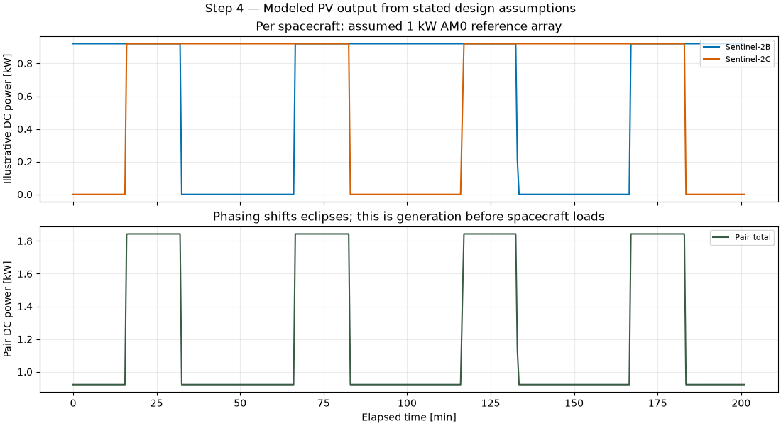
Sentinel-2B design position: illustrative 24 h DC energy 14.84 kWh; mean Sun visibility 67.1%
Sentinel-2C design position: illustrative 24 h DC energy 14.60 kWh; mean Sun visibility 66.0%
Total running time of the script: (0 minutes 1.009 seconds)