Note
Go to the end to download the full example code.
Healthy reference calibration with an explicit Gaussian posterior#
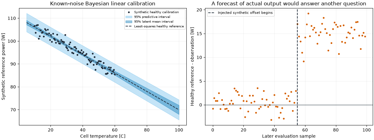
This is a controlled synthetic experiment: an independently designated healthy training run calibrates a temperature-power reference. A later measurement sequence contains a deliberately injected offset. The fitted reference predicts healthy expectation; it is not trained to reproduce the degraded operating sequence.
The conjugate Bayesian linear calculation uses stated noise and prior assumptions. It is neither a neural digital twin nor a full reproduction of a mission paper. Credible/predictive intervals require the Gaussian linear assumptions; uncertainty from missing physics remains outside this model.
import matplotlib.pyplot as plt
import numpy as np
import pandas as pd

import orbitalpv as opv
rng = np.random.default_rng(42)
temperature = np.linspace(10, 60, 80)
training_power = 100 - 0.4 * (temperature - 25) + rng.normal(0, 2, len(temperature))
training_times = pd.date_range("2026-01-01", periods=len(temperature), freq="min", tz="UTC")
reference = opv.fit_bayesian_linear_calibration(
    temperature,
    training_power,
    timestamps=training_times,
    purpose="healthy_reference",
    evidence="Synthetic controlled healthy run; no flight validation claimed",
    observation_noise_std=2.0,
    prior_std=100,
)
deterministic = opv.fit_linear_calibration(
    temperature,
    training_power,
    timestamps=training_times,
    purpose="healthy_reference",
    evidence="Same independently designated synthetic healthy training run",
)
evaluation_temperature = np.linspace(5, 100, 100)
evaluation_times = pd.date_range("2026-01-02", periods=100, freq="min", tz="UTC")
prediction = reference.predict(evaluation_temperature, timestamps=evaluation_times, coverage=0.95)
latent = reference.predict(
    evaluation_temperature,
    timestamps=evaluation_times,
    coverage=0.95,
    include_observation_noise=False,
)
actual = 100 - 0.4 * (evaluation_temperature - 25) + rng.normal(0, 2, 100)
actual[55:] -= 15

fig, axes = plt.subplots(1, 2, figsize=(12, 4.5), layout="constrained")
axes[0].plot(
    temperature, training_power, ".", color="#202C39", label="Synthetic healthy calibration"
)
axes[0].fill_between(
    evaluation_temperature,
    prediction.lower,
    prediction.upper,
    color="#56B4E9",
    alpha=0.35,
    label="95% predictive interval",
)
axes[0].fill_between(
    evaluation_temperature,
    latent.lower,
    latent.upper,
    color="#0072B2",
    alpha=0.4,
    label="95% latent mean interval",
)
axes[0].plot(
    evaluation_temperature,
    deterministic.predict(evaluation_temperature)[:, 0],
    "--",
    color="#202C39",
    label="Least-squares healthy reference",
)
axes[0].set(
    xlabel="Cell temperature [C]",
    ylabel="Synthetic reference power [W]",
    title="Known-noise Bayesian linear calibration",
)
axes[0].legend(fontsize=7)

residual = prediction["mean"].to_numpy() - actual
axes[1].plot(np.arange(100), residual, ".", color="#D55E00")
axes[1].axvline(55, color="#202C39", linestyle="--", label="Injected synthetic offset begins")
axes[1].axhline(0, color="#202C39", linewidth=0.8)
axes[1].set(
    xlabel="Later evaluation sample",
    ylabel="Healthy reference - observation [W]",
    title="A forecast of actual output would answer another question",
)
axes[1].legend(fontsize=8)
for ax in axes:
    ax.grid(alpha=0.2)
plt.show()
print("Posterior coefficient covariance:", reference.coefficient_covariance)
Posterior coefficient covariance: [[ 4.99997500e-02 -8.04903644e-18]
 [-8.04903644e-18  4.99997500e-02]]
Total running time of the script: (0 minutes 0.221 seconds)