Note
Go to the end to download the full example code.
SpaceX Starmind: from HJT solar cells to usable orbital compute#
The November 11, 2026 BigGo report motivates this scenario. SINGULUS confirms an HJT manufacturing agreement; SpaceX lists AI1 at 175 kW average and 250 kW peak compute. Every other hardware and operating input below is an explicit assumption in the checked-in JSON, with primary-source links and evidence status.
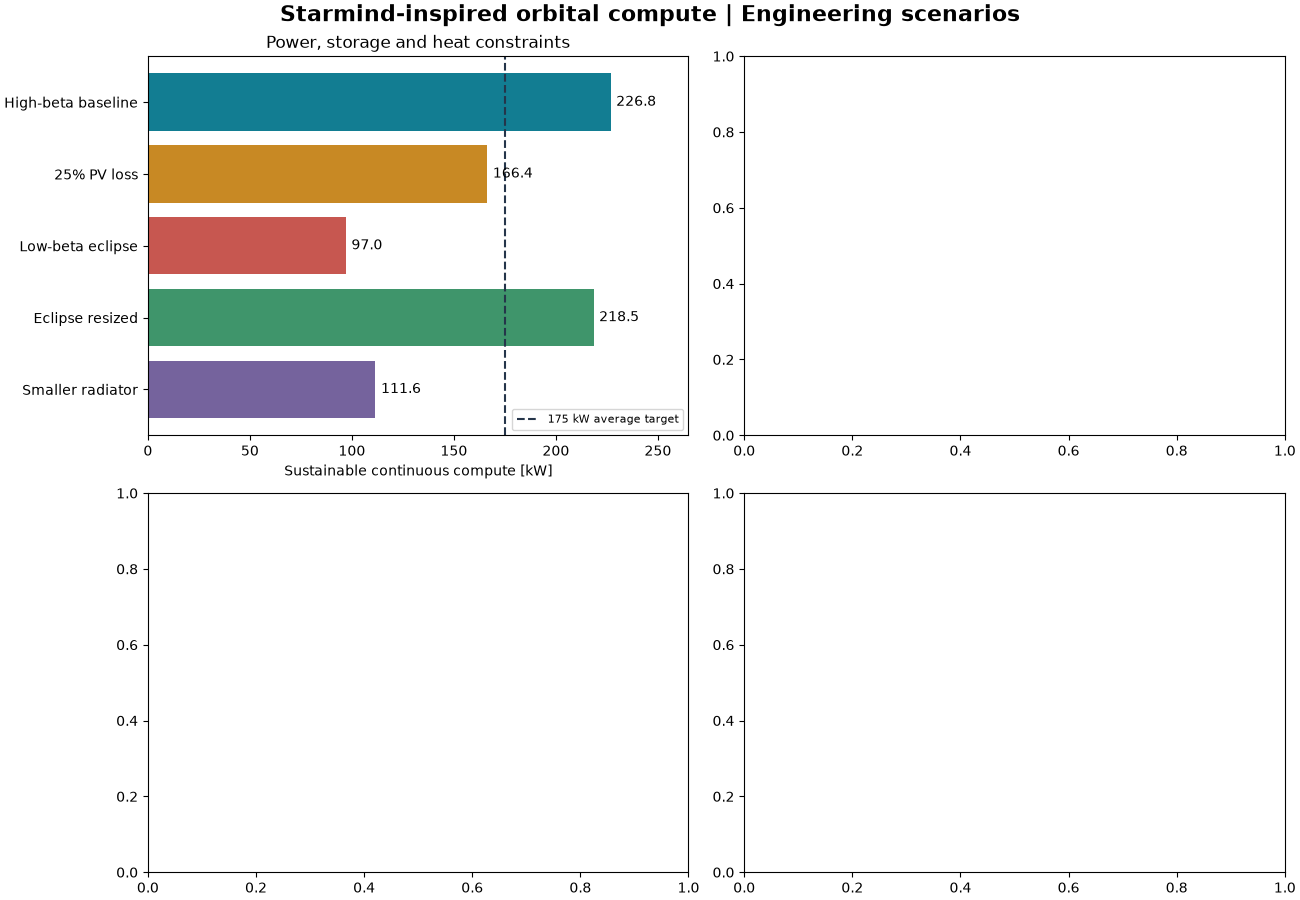
Decision: how much continuous computing survives eclipse, PV loss and radiator constraints, and how does the 100 GW/year ambition compare with launch throughput? These are synthetic scenarios, not SpaceX specifications or measured performance.
Run python analysis/spacex_starmind/run.py for CSV traces, provenance and
sensitivity tables. Requires an installed source checkout and matplotlib.
import json
from dataclasses import replace
from pathlib import Path

import matplotlib.pyplot as plt
import numpy as np

from orbitalpv.orbital_compute import (
    OrbitalComputeSpec,
    deployment_screen,
    screen_orbital_compute,
    simulate_orbital_compute,
)
from orbitalpv.physics import BatterySpec

directory = Path(__file__).resolve().parent if "__file__" in globals() else Path.cwd()
data = json.loads((directory / "_data/spacex_starmind.json").read_text())
baseline = dict(data["baseline"])
battery = BatterySpec(**baseline.pop("battery"))
base = OrbitalComputeSpec(**baseline, battery=battery)
specs = [
    replace(base, **s["changes"], battery=replace(base.battery, **s.get("battery_changes", {})))
    for s in data["scenarios"]
]
screens = [screen_orbital_compute(s) for s in specs]
colors = ["#127D92", "#C88924", "#C75750", "#3F956B", "#75639D"]
fig, axes = plt.subplots(2, 2, figsize=(13, 9), layout="constrained")
fig.suptitle(
    "Starmind-inspired orbital compute | Engineering scenarios", fontsize=16, weight="bold"
)
ax = axes[0, 0]
names = [s["name"] for s in data["scenarios"]]
capacity = [float(s["sustainable_compute_kw"]) for s in screens]
bars = ax.barh(names, capacity, color=colors)
ax.bar_label(bars, fmt="%.1f", padding=4)
ax.axvline(175, color="#25354A", linestyle="--", label="175 kW average target")
ax.invert_yaxis()
ax.set(
    xlabel="Sustainable continuous compute [kW]",
    xlim=(0, 265),
    title="Power, storage and heat constraints",
)
ax.legend(loc="lower right", fontsize=8)
<matplotlib.legend.Legend object at 0x790bc7dbe5d0>
ax = axes[0, 1]
for i in (0, 2, 3):
    trace = simulate_orbital_compute(specs[i])
    tail = trace[trace.cycle >= 38]
    time = (tail.interval_start_s - tail.interval_start_s.iloc[0]) / 3600
    ax.step(time, tail.served_compute_w / 1000, where="post", color=colors[i], label=names[i])
    if i == 0:
        ax.step(
            time,
            tail.requested_compute_w / 1000,
            where="post",
            linestyle="--",
            color="#25354A",
            label="Requested",
        )
ax.set(
    xlabel="Time in final two orbits [h]",
    ylabel="Compute served [kW]",
    title="250 kW bursts: actual served power",
)
ax.legend(fontsize=8, loc="lower left")
<matplotlib.legend.Legend object at 0x790bc84fa990>
ax = axes[1, 0]
beta = np.linspace(0, 90, 91)
for area, battery_kwh, color in ((1000, 100, colors[0]), (1600, 240, colors[3])):
    power = [
        screen_orbital_compute(
            replace(
                base,
                beta_angle_deg=float(b),
                pv_area_m2=area,
                battery=replace(base.battery, capacity_wh=battery_kwh * 1000),
            )
        )["sustainable_compute_kw"]
        for b in beta
    ]
    ax.plot(beta, power, label=f"{area} m² PV / {battery_kwh} kWh", color=color, linewidth=2)
ax.axhline(175, color="#25354A", linestyle="--")
ax.set(
    xlabel="Absolute orbit beta angle [degrees]",
    ylabel="Continuous compute [kW]",
    title="Eclipse sensitivity at assumed 550 km",
)
ax.legend(fontsize=8)
<matplotlib.legend.Legend object at 0x790bc8488f50>
ax = axes[1, 1]
launches = np.arange(0, 10001, 250)
added_compute = [
    deployment_screen(
        **{**data["deployment"], "launches_per_year": int(n)},
        array_area_m2=base.pv_area_m2,
        continuous_compute_kw=175,
    )["added_continuous_compute_gw"]
    for n in launches
]
ax.plot(launches, added_compute, color=colors[0], linewidth=2)
ax.scatter([1000], [3.5], color=colors[2], zorder=3)
ax.annotate(
    "1,000 assumed launches → 3.5 GW",
    (1000, 3.5),
    xytext=(1500, 6),
    fontsize=9,
    arrowprops={"arrowstyle": "->", "color": colors[2]},
)
ax.set(
    xlabel="Assumed launches to target orbit per year",
    ylabel="Added continuous compute [GW]",
    title="100 GW/year factory scenario; mass-only launch cap",
)
for ax in axes.flat:
    ax.grid(alpha=0.15, axis="x")
    ax.spines[["top", "right"]].set_visible(False)
plt.show()
The 100 GW/year manufacturing case assumes an STC basis, 80% utilization, 90% yield and 50% space allocation. It is not contracted first-line capacity. Launch inputs are hypothetical: 5 t complete spacecraft, 100 t payload to the target orbit, 1,000 flights/year. No fairing or orbital approval is implied. Electrical energy served is not tokens/s, FLOPS, training throughput, revenue or proof of chip-temperature feasibility. Those require additional models.
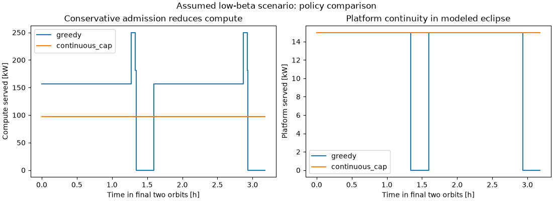
This is conservative admission control under the same assumed repeating orbit, not a flight controller or a prediction of useful AI work. Rejected work is lost.
fig_policy, axes_policy = plt.subplots(1, 2, figsize=(11, 4), layout="constrained")
for policy in ("greedy", "continuous_cap"):
    trace = simulate_orbital_compute(specs[2], dispatch_policy=policy)
    tail = trace[trace.cycle >= 38]
    time = (tail.interval_start_s - tail.interval_start_s.iloc[0]) / 3600
    axes_policy[0].step(time, tail.served_compute_w / 1000, where="post", label=policy)
    axes_policy[1].step(time, tail.served_platform_w / 1000, where="post", label=policy)
axes_policy[0].set(ylabel="Compute served [kW]", title="Conservative admission reduces compute")
axes_policy[1].set(ylabel="Platform served [kW]", title="Platform continuity in modeled eclipse")
for ax in axes_policy:
    ax.set_xlabel("Time in final two orbits [h]")
    ax.legend()
fig_policy.suptitle("Assumed low-beta scenario: policy comparison")
plt.show()
Total running time of the script: (0 minutes 0.715 seconds)