Note
Go to the end to download the full example code.
Expected versus actual power with known operating states#
Build an operating loss ledger for two explicitly simulated spacecraft arrays. The healthy operating expectation already contains Earth eclipse, planned incidence, and cell temperature. Additional stages represent supplied actual pointing, a known retention adjustment, a controller limit, and availability. These cumulative predictions are compared with synthetic telemetry; their remaining difference stays unexplained.
This differs from an ideal-reference design waterfall. Normal eclipse and temperature effects are already in the starting expectation here, so adding their full losses again would double-count them. The two arrays also have different data gaps: energy results cover accepted observed intervals only.
Evidence and assumptions#
Every input is generated locally for demonstration, including the telemetry and the evidence labels. No spacecraft fault or measured flight result is claimed. A circular 550 km orbit and a fixed Sun at 1 AU provide illumination. The two array references are 40 W and 30 W at 1361 W/m² and 25°C. Planned incidence angles are 20 and 35 degrees. Their actual attitudes, temperatures, retention factors, and controller states are declared synthetic inputs.
The final synthetic power includes an omitted shortfall and signed sensor noise, so the residual contains both losses and gains. No algorithm is asked to infer their causes. Missing measurements and a missing pointing input are retained as NaNs; an additional telemetry outage has no records at all.
Relevant primary guidance:
NASA normalized illumination and temperature and selected peak-power operation before assessing an array’s degradation: https://ntrs.nasa.gov/citations/19850025862
NASA’s ISS study used shunt-current evidence because delivered array power was also governed by load demand: https://ntrs.nasa.gov/citations/20050215410
Power sampling conventions and interpolation limits matter for energy: https://rdtools.readthedocs.io/en/stable/generated/rdtools.normalization.energy_from_power.html
from itertools import pairwise

import matplotlib.pyplot as plt
import numpy as np
import pandas as pd

import orbitalpv as opv
The artificial UTC epoch only labels this simulation; these are not flight ephemerides. Keep a finite solar disc and realistic eclipse edges, but freeze the Sun over three orbits. The electrical boundary is each array’s DC output under its controller’s operating point, before any downstream converter.
MAX_GAP_S = 75.0
epoch = pd.Timestamp("2025-06-01T00:00:00Z")
altitude_m = 550_000.0
period_s = opv.circular_orbit_period_s(altitude_m)
cadences_s = np.resize(np.array([29.0, 31.0, 34.0, 27.0, 33.0, 30.0]), 700)
elapsed_s = np.r_[0.0, np.cumsum(cadences_s)]
elapsed_s = elapsed_s[elapsed_s <= 3.0 * period_s]
minutes = elapsed_s / 60.0
phase = elapsed_s * 2.0 * np.pi / period_s
positions_m = opv.keplerian_orbit_positions_m(
    opv.EARTH_EQUATORIAL_RADIUS_M + altitude_m,
    0.0,
    51.6,
    raan_deg=30.0,
    true_anomaly_rad=phase,
)
sun_position_m = np.array([opv.ASTRONOMICAL_UNIT_M, 0.0, 0.0])
illumination = np.array(
    [opv.earth_occultation_fraction(position, sun_position_m) for position in positions_m]
)

rng = np.random.default_rng(41)
frames = []
for panel_id, rating_w, planned_angle_deg, retention, offset in (
    ("Array A", 40.0, 20.0, 0.970, 0.0),
    ("Array B", 30.0, 35.0, 0.985, 0.7),
):
    temperature_c = 25.0 + 24.0 * (0.5 + 0.5 * np.sin(phase - 0.7 + offset))
    reference = opv.PvwattsReference(
        pdc0_w=rating_w,
        gamma_pdc_per_c=-0.003,
        reference_irradiance_w_m2=1361.0,
        reference_temperature_c=25.0,
    )
    planned_cosine = np.cos(np.deg2rad(planned_angle_deg))
    expected_w = opv.pvwatts_dc_space(
        1361.0 * illumination * planned_cosine, temperature_c, reference
    )

    # Actual pointing can be better or worse than the planned incidence. Its
    # contribution is therefore allowed to be a gain. Temperature and eclipse
    # remain the same observed/supplied inputs in both predictions.
    actual_angle_deg = 20.0 + 18.0 * np.sin(2.0 * np.pi * minutes / 72.0 + offset)
    after_pointing_w = expected_w * np.cos(np.deg2rad(actual_angle_deg)) / planned_cosine
    after_retention_w = after_pointing_w * retention
    cap_w = 22.0 if panel_id == "Array A" else 18.0
    limit_w = np.where((minutes >= 70.0) & (minutes <= 90.0), cap_w, np.inf)
    after_limit_w = np.minimum(after_retention_w, limit_w)
    available = ~((minutes >= 175.0) & (minutes <= 181.0))
    modeled_truth_w = after_limit_w * available

    # This omitted effect is deliberately NOT passed as a diagnostic stage.
    # The ledger must leave it, together with sensor noise, unexplained.
    omitted_shortfall_w = np.where((minutes >= 198.0) & (minutes <= 205.0), 2.5, 0.0)
    actual_w = modeled_truth_w - omitted_shortfall_w + rng.normal(0.0, 0.18, len(minutes))
    actual_w[(minutes >= 23.0) & (minutes <= 26.0)] = np.nan
    supplied_pointing_w = after_pointing_w.copy()
    supplied_pointing_w[(minutes >= 264.0) & (minutes <= 267.0)] = np.nan

    frame = pd.DataFrame(
        {
            "timestamp": epoch + pd.to_timedelta(elapsed_s, unit="s"),
            "panel_id": panel_id,
            "expected_power_w": expected_w,
            "after_pointing_w": supplied_pointing_w,
            "after_retention_w": after_retention_w,
            "after_limit_w": after_limit_w,
            "after_availability_w": modeled_truth_w,
            "actual_power_w": actual_w,
        }
    )
    outage_end_min = 119.0 if panel_id == "Array A" else 129.0
    frame = frame.loc[~((minutes >= 108.0) & (minutes <= outage_end_min))]
    frames.append(frame)
telemetry = pd.concat(frames, ignore_index=True)

stages = (
    opv.LossStage(
        name="pointing",
        power_column="after_pointing_w",
        category="geometry",
        evidence="Synthetic supplied actual attitude versus planned incidence",
    ),
    opv.LossStage(
        name="retention",
        power_column="after_retention_w",
        category="degradation",
        evidence="Declared synthetic retention factors 0.970 and 0.985; not fitted from residuals",
    ),
    opv.LossStage(
        name="controller_limit",
        power_column="after_limit_w",
        category="operations",
        evidence="Synthetic commanded array-output limits from minute 70 to 90",
    ),
    opv.LossStage(
        name="availability",
        power_column="after_availability_w",
        category="operations",
        evidence="Synthetic controller disconnect flag from minute 175 to 181",
    ),
)
breakdown = opv.power_loss_breakdown(telemetry, stages, group_columns=("panel_id",))
summary = opv.summarize_power_losses(breakdown, max_gap_s=MAX_GAP_S)
samples = breakdown.samples.copy()
samples["elapsed_min"] = (samples["timestamp"] - epoch).dt.total_seconds() / 60.0


def observed_slices(times_min):
    """Plot separate recorded blocks, without drawing across the long outage."""
    boundaries = np.r_[0, np.flatnonzero(np.diff(times_min) * 60.0 > MAX_GAP_S) + 1, len(times_min)]
    return [slice(left, right) for left, right in pairwise(boundaries)]


def plot_observed(ax, times_min, values, *, label, **kwargs):
    for index, block in enumerate(observed_slices(times_min)):
        ax.plot(times_min[block], values[block], label=label if index == 0 else None, **kwargs)


fig, axes = plt.subplots(2, 1, figsize=(11, 7), sharex=True, layout="constrained")
for ax, (panel_id, panel) in zip(axes, samples.groupby("panel_id", sort=False), strict=True):
    times_min = panel["elapsed_min"].to_numpy()
    for column, label, color, style in (
        ("expected_power_w", "Healthy operating expectation", "#333333", "-"),
        ("modeled_power_w", "After supplied operating adjustments", "#0072B2", "--"),
        ("actual_power_w", "Synthetic actual telemetry", "#D55E00", "-"),
    ):
        plot_observed(
            ax,
            times_min,
            panel[column].to_numpy(),
            label=label,
            color=color,
            linestyle=style,
            linewidth=1.1,
        )
    ax.set(ylabel="DC power [W]", title=panel_id)
    ax.grid(alpha=0.22)
axes[0].legend(fontsize=8, loc="upper right")
axes[-1].set(xlabel="Minutes from synthetic UTC epoch", xlim=(0, minutes[-1]))
fig.suptitle("Step 1 — Compare at the same operating point and electrical boundary")
plt.show()
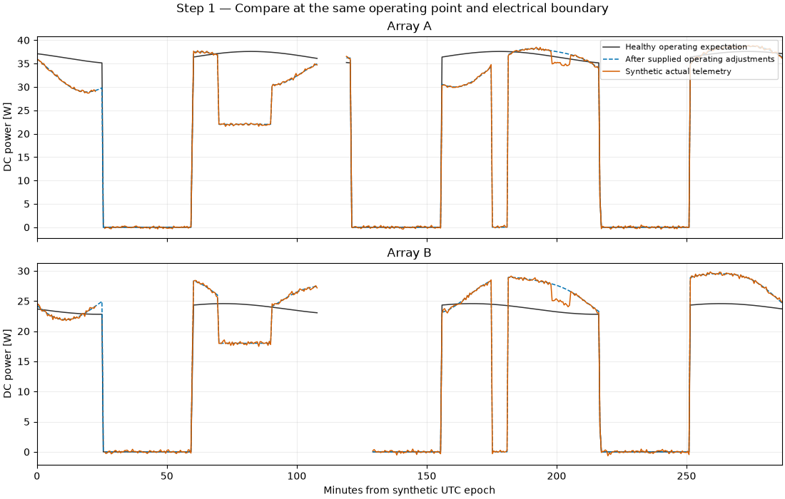
A category is a reporting bucket, not a causal classifier. Two independently supplied controller stages combine under operations; the final remainder is never redistributed among the physical categories. Losses are positive and gains negative. Gaps also appear when any required input is missing.
panel = samples[samples["panel_id"].eq("Array A")]
times_min = panel["elapsed_min"].to_numpy()
category_labels = {
    "geometry": "Actual versus planned pointing",
    "degradation": "Supplied retention adjustment",
    "operations": "Known limits and availability",
    "unexplained": "Unexplained model-minus-telemetry residual",
}
fig, axes = plt.subplots(4, 1, figsize=(11, 9), sharex=True, layout="constrained")
for ax, (category, title) in zip(axes, category_labels.items(), strict=True):
    values = breakdown.categories_w.loc[panel.index, category].to_numpy()
    for block in observed_slices(times_min):
        ax.fill_between(
            times_min[block],
            0,
            values[block],
            where=values[block] >= 0,
            color="#D55E00",
            alpha=0.55,
        )
        ax.fill_between(
            times_min[block], 0, values[block], where=values[block] < 0, color="#0072B2", alpha=0.55
        )
    ax.axhline(0.0, color="#444444", linewidth=0.7)
    ax.set(ylabel="Signed loss [W]", title=title)
    ax.grid(alpha=0.2)
axes[-1].set(xlabel="Minutes from synthetic UTC epoch", xlim=(0, minutes[-1]))
fig.suptitle("Step 2 — Array A: orange losses, blue gains, and explicit missing intervals")
plt.show()
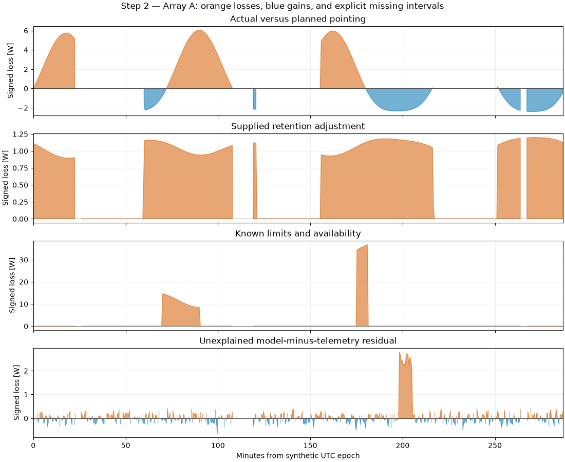
Every bar uses the same valid adjacent samples with a gap limit of 75 s. The energy waterfall is for Array A only. It is not an extrapolation to the unobserved hours, nor a fleet total mixing the two arrays’ different coverage. The contribution order is the stage order, so interactions are accounted for once. These are sequential contributions, not independent sensitivity tests.
total = summary.totals.set_index("panel_id").loc["Array A"]
components = summary.components[summary.components["panel_id"].eq("Array A")]
stage_labels = {
    "pointing": "Pointing",
    "retention": "Retention",
    "controller_limit": "Controller\nlimit",
    "availability": "Availability",
    "unexplained": "Unexplained",
}
fig, ax = plt.subplots(figsize=(11, 5.6), layout="constrained")
start_energy = float(total["expected_energy_wh"])
actual_energy = float(total["actual_energy_wh"])
ax.bar(0, start_energy, width=0.7, color="#555555")
ax.text(0, start_energy, f"{start_energy:.2f}", ha="center", va="bottom")
level = start_energy
tick_labels = ["Operating\nexpectation"]
for index, row in enumerate(components.itertuples(), start=1):
    loss = row.net_loss_wh
    next_level = level - loss
    color = "#D55E00" if loss >= 0 else "#0072B2"
    ax.plot([index - 1 + 0.35, index - 0.35], [level, level], color="#777777", linewidth=0.8)
    ax.bar(index, abs(loss), bottom=min(level, next_level), width=0.7, color=color)
    ax.text(index, max(level, next_level) + 1, f"{loss:+.2f}", ha="center", fontsize=9)
    tick_labels.append(stage_labels[row.component])
    level = next_level
last_index = len(components) + 1
ax.plot([last_index - 1 + 0.35, last_index - 0.35], [level, level], color="#777777", linewidth=0.8)
ax.bar(last_index, actual_energy, width=0.7, color="#009E73")
ax.text(last_index, actual_energy, f"{actual_energy:.2f}", ha="center", va="bottom")
tick_labels.append("Synthetic\nactual")
ax.set(
    xticks=np.arange(len(tick_labels)),
    xticklabels=tick_labels,
    ylabel="Energy on accepted observed intervals [Wh]",
    title=(
        "Step 3 — Array A: signed contributions reconcile expected and actual energy\n"
        f"{total['observed_duration_h']:.2f} h observed; {total['coverage_fraction']:.1%} "
        "of the recorded window"
    ),
    ylim=(0, max(start_energy, actual_energy) * 1.16),
)
ax.grid(axis="y", alpha=0.22)
ax.set_axisbelow(True)
plt.show()
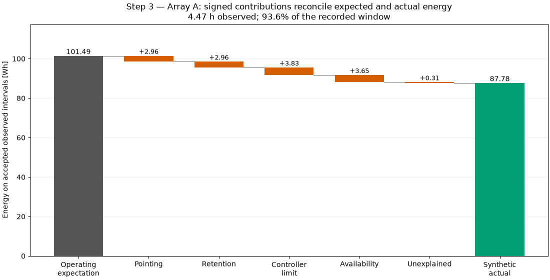
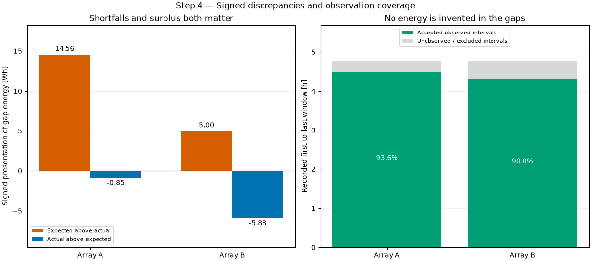
Positive gap and surplus are areas of the total expected-minus-actual curve, integrated with exact linear zero crossings. They are not the separate sum of every component’s positive and negative area: components can cancel. Coverage is per array and only spans its first to last recorded timestamp.
totals = summary.totals.set_index("panel_id")
x = np.arange(len(totals))
fig, axes = plt.subplots(1, 2, figsize=(12, 5.3), layout="constrained")
positive = axes[0].bar(
    x - 0.18,
    totals["positive_gap_energy_wh"],
    width=0.36,
    color="#D55E00",
    label="Expected above actual",
)
negative = axes[0].bar(
    x + 0.18,
    -totals["surplus_energy_wh"],
    width=0.36,
    color="#0072B2",
    label="Actual above expected",
)
axes[0].bar_label(positive, fmt="%.2f", padding=3)
axes[0].bar_label(negative, fmt="%.2f", padding=3)
axes[0].axhline(0, color="#555555", linewidth=0.8)
axes[0].set(
    ylabel="Signed presentation of gap energy [Wh]", title="Shortfalls and surplus both matter"
)
axes[0].legend(fontsize=8, loc="lower left")
axes[0].margins(y=0.18)
axes[1].bar(x, totals["observed_duration_h"], color="#009E73", label="Accepted observed intervals")
axes[1].bar(
    x,
    totals["window_duration_h"] - totals["observed_duration_h"],
    bottom=totals["observed_duration_h"],
    color="#D8D8D8",
    label="Unobserved / excluded intervals",
)
for index, (_, row) in enumerate(totals.iterrows()):
    axes[1].text(
        index,
        row["observed_duration_h"] / 2,
        f"{row['coverage_fraction']:.1%}",
        ha="center",
        color="white",
    )
axes[1].set(ylabel="Recorded first-to-last window [h]", title="No energy is invented in the gaps")
axes[1].legend(fontsize=8, loc="upper center")
axes[1].set_ylim(0, float(totals["window_duration_h"].max()) * 1.19)
for ax in axes:
    ax.set_xticks(x, totals.index)
    ax.grid(axis="y", alpha=0.2)
    ax.set_axisbelow(True)
fig.suptitle("Step 4 — Signed discrepancies and observation coverage")
plt.show()

valid = breakdown.samples["valid"]
sample_closure_w = (
    (breakdown.components_w.loc[valid].sum(axis=1) - breakdown.samples.loc[valid, "total_loss_w"])
    .abs()
    .max()
)
print("All telemetry and operating inputs in this example are synthetic.")
print(f"Maximum sample ledger closure error: {sample_closure_w:.3g} W")
print(f"Array A waterfall closure error: {level - actual_energy:.3g} Wh")
print(
    summary.totals[
        [
            "panel_id",
            "expected_energy_wh",
            "actual_energy_wh",
            "gap_energy_wh",
            "unexplained_energy_wh",
            "observed_duration_h",
            "coverage_fraction",
            "valid_intervals",
        ]
    ].to_string(index=False, float_format=lambda value: f"{value:.3f}")
)
All telemetry and operating inputs in this example are synthetic.
Maximum sample ledger closure error: 0 W
Array A waterfall closure error: 0 Wh
panel_id  expected_energy_wh  actual_energy_wh  gap_energy_wh  unexplained_energy_wh  observed_duration_h  coverage_fraction  valid_intervals
 Array A             101.489            87.780         13.709                  0.313                4.472              0.936              525
 Array B              65.112            65.996         -0.884                  0.285                4.302              0.900              505
Total running time of the script: (0 minutes 0.938 seconds)