Note
Go to the end to download the full example code.
Measured GOES proton and electron environment#
Retrieve seven days of actual GOES particle measurements from NOAA SWPC, inspect sampling coverage, and compare the measured integral energy channels. These observations describe the environment at the reporting geostationary spacecraft. They are not solar-panel electrical output or a radiation dose for another satellite. Computing solar-cell damage needs an orbit, shielding, particle spectrum and a separately validated damage model.
Sources:
NOAA supplies five-minute integral flux in particles/(cm² s sr). Preserve each record’s satellite identity: the primary proton and electron instruments can be on different spacecraft. Integral channels overlap, so their fluxes must not be summed. Electron measurements can be contaminated by energetic protons; this feed has no per-record flag that establishes contamination.
This is a rolling recent-data service. The first run retrieves the current
window; subsequent runs reuse the exact cached responses and their checksum
sidecars. Use refresh=True to replace those snapshots. The printed times
and retrieval metadata identify the data used by this particular build.
from pathlib import Path
from tempfile import gettempdir

import matplotlib.pyplot as plt
import pandas as pd

import orbitalpv as opv
cache = Path(gettempdir()) / "orbitalpv-real-data" / "goes"
with opv.NoaaSwpcConnector() as connector:
    protons = connector.goes_integral_particle_flux(
        "protons", cache_path=cache / "protons-7-day.json"
    )
    electrons = connector.goes_integral_particle_flux(
        "electrons", cache_path=cache / "electrons-7-day.json"
    )

for name, frame in [("protons", protons), ("electrons", electrons)]:
    print(
        f"{name}: {len(frame):,} channel observations; {frame['timestamp'].nunique():,} measurement times"
    )
    print(f"UTC range: {frame['timestamp'].min()} to {frame['timestamp'].max()}")
    print(f"Sources: {', '.join(frame['satellite_id'].unique())}")
    print(f"Retrieved: {frame.attrs['retrieved_at']}; SHA256: {frame.attrs['sha256']}")

flux = pd.concat([protons, electrons], ignore_index=True)
coverage = flux.groupby(["particle", "satellite_id", "energy"], as_index=False).agg(
    observations=("timestamp", "size"), valid_flux=("is_valid_flux", "sum")
)
labels = coverage["satellite_id"] + " " + coverage["particle"] + " " + coverage["energy"]
fig, ax = plt.subplots(figsize=(10, 5), layout="constrained")
ax.barh(labels, coverage["observations"], label="Reported", color="#BEC9D8")
ax.barh(labels, coverage["valid_flux"], label="Valid flux", color="#0072B2")
ax.set(xlabel="Observations", title="Step 1 — Measurement coverage by source and energy threshold")
ax.grid(True, axis="x", alpha=0.25)
ax.legend()
plt.show()
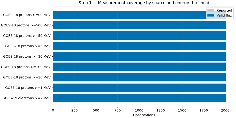
protons: 16,104 channel observations; 2,013 measurement times
UTC range: 2026-11-08 03:00:00+00:00 to 2026-11-15 02:50:00+00:00
Sources: GOES-18
Retrieved: 2026-11-15T03:00:53.065169+00:00; SHA256: 584b95d34423eb91d183844c83854f2dd3d3e77e775940146d599c0af8d63945
electrons: 2,013 channel observations; 2,013 measurement times
UTC range: 2026-11-08 03:00:00+00:00 to 2026-11-15 02:50:00+00:00
Sources: GOES-19
Retrieved: 2026-11-15T03:00:53.130366+00:00; SHA256: 9e9c702c50e75f6bcd1a11bac3d7a7de090ece7b8405847ee4e57dacacb123d9
Plot actual timestamps as markers, leaving gaps unfilled. A logarithmic axis displays the different flux scales. Zero and invalid fluxes are omitted from this log plot; the coverage summary above still accounts for them.
fig, ax = plt.subplots(figsize=(10, 5), layout="constrained")
for (satellite, energy), group in protons.groupby(["satellite_id", "energy_threshold_mev"]):
    shown = group[group["flux_cm2_s_sr"] > 0]
    ax.plot(
        shown["timestamp"],
        shown["flux_cm2_s_sr"],
        ".",
        ms=2,
        alpha=0.65,
        label=f"{satellite}, ≥{energy:g} MeV",
    )
ax.set(
    yscale="log",
    xlabel="UTC observation time",
    ylabel="Integral proton flux [cm⁻² s⁻¹ sr⁻¹]",
    title="Step 2 — Measured GOES proton environment",
)
ax.grid(True, alpha=0.25)
ax.legend(fontsize=7, ncols=2)
fig.autofmt_xdate()
plt.show()
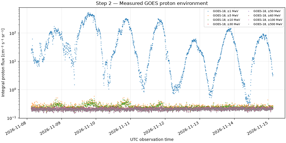
Retaining the original spacecraft identifier prevents a primary-role change from being mistaken for one uninterrupted instrument record. These measured fluxes can support a separate environment study, but are not directly comparable to BIRDS or Flying Laptop panel output without a physical model.
fig, ax = plt.subplots(figsize=(10, 4.5), layout="constrained")
for (satellite, energy), group in electrons.groupby(["satellite_id", "energy_threshold_mev"]):
    shown = group[group["flux_cm2_s_sr"] > 0]
    ax.plot(
        shown["timestamp"], shown["flux_cm2_s_sr"], ".", ms=2, label=f"{satellite}, ≥{energy:g} MeV"
    )
ax.set(
    yscale="log",
    xlabel="UTC observation time",
    ylabel="Integral electron flux [cm⁻² s⁻¹ sr⁻¹]",
    title="Step 3 — Measured GOES electron environment",
)
ax.grid(True, alpha=0.25)
ax.legend()
fig.autofmt_xdate()
plt.show()
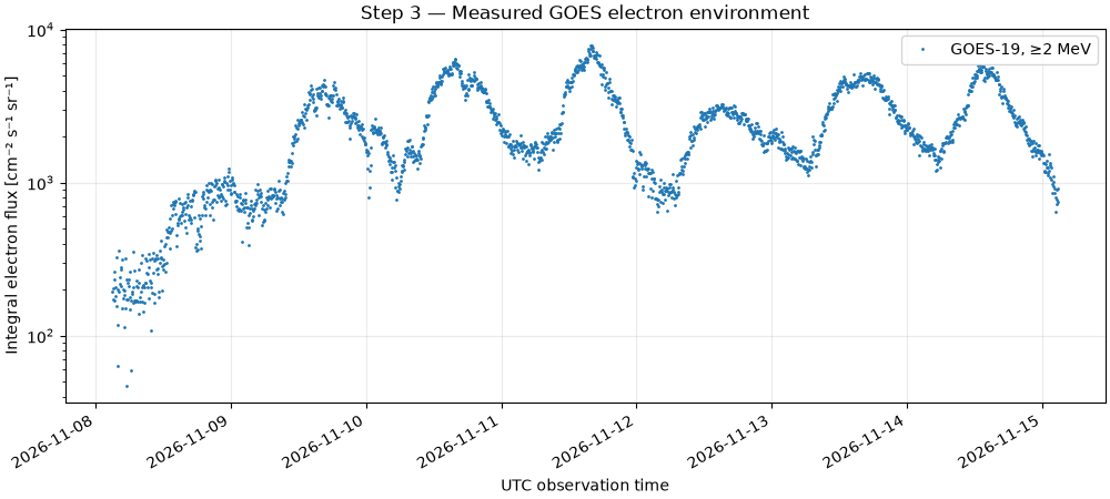
Total running time of the script: (0 minutes 1.091 seconds)