Note
Go to the end to download the full example code.
Ground imagery and mapped solar-farm inputs#
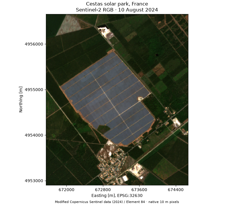
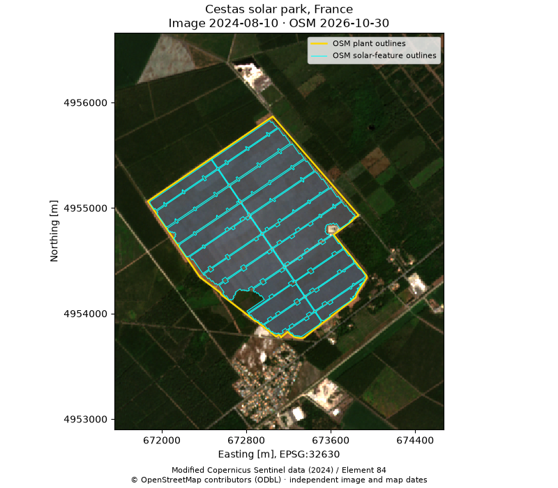
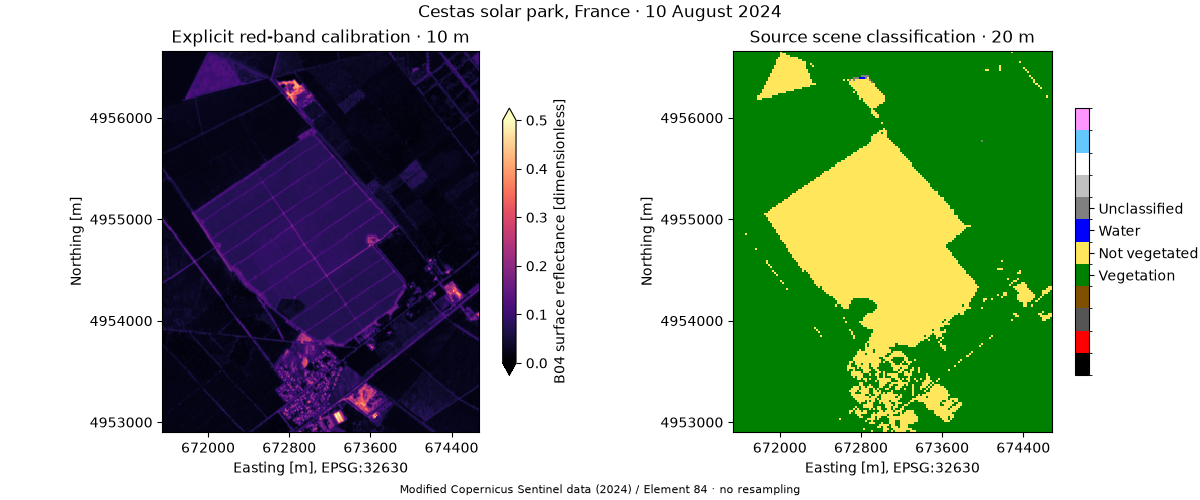
Inspect Cestas, France, with the shared PV mapping utilities. One call loads verified Sentinel-2 crops and the original OpenStreetMap (OSM) features; the plotting helpers produce RGB, mapped outlines and spectral-quality views.
Dunnett et al. (2020) builds its inventory from OSM. These utilities prepare those source features and add image context; the companion footprint and inventory examples demonstrate image classification, farm grouping and calibrated capacity estimates. The image is from 10 August 2024, while the OSM snapshot is from 30 October 2026. The outlines are not contemporaneous validation labels.
Contains modified Copernicus Sentinel data (2024), processed by Element 84; OSM data © OpenStreetMap contributors, ODbL-1.0.
Install the repository with its ground,examples extras. Bundled real
snapshots run offline; set ORBITALPV_GROUND_LIVE=1 to fetch a separate
copy. The downloaded script also fetches when its companion folder is absent.
See _data/README.txt for provenance and data-license details.
import os
from pathlib import Path
from pprint import pprint
from tempfile import gettempdir

import matplotlib.pyplot as plt

import orbitalpv as opv
example_dir = Path(__file__).resolve().parent if "__file__" in globals() else Path.cwd()
bundled = example_dir / "_data"
live = os.environ.get("ORBITALPV_GROUND_LIVE") == "1" or not bundled.is_dir()
site = opv.load_pv_site(
    name="Cestas solar park, France",
    bbox=(-0.833, 44.709, -0.795, 44.742),
    time_min="2024-06-01",
    time_max="2024-09-01",
    max_cloud_cover=10,
    max_items=10,
    cache_dir=Path(gettempdir()) / "orbitalpv-ground-cestas" if live else bundled,
    cache_prefix="cestas",
    offline=not live,
)
pprint(site.summary(), sort_dicts=False)
{'name': 'Cestas solar park, France',
 'bbox_wgs84': [-0.833, 44.709, -0.795, 44.742],
 'scene_id': 'S2A_T30TXQ_20240810T105747_L2A',
 'acquired_at': '2024-08-10T11:08:48.933000Z',
 'scene_cloud_cover_percent': 0.031728,
 'search': {'returned': 3, 'matched': 3, 'limit': 10, 'limit_reached': False},
 'osm_timestamp': '2026-10-30T08:24:41Z',
 'osm_element_counts': {'way': 23},
 'images': {'visual': {'shape': [3, 376, 312],
                       'dtype': 'uint8',
                       'crs': 'EPSG:32630',
                       'pixel_size': [10.0, 10.0],
                       'bounds': [671550.0, 4952900.0, 674670.0, 4956660.0],
                       'masked_band_samples': 9},
            'red': {'shape': [1, 376, 312],
                    'dtype': 'uint16',
                    'crs': 'EPSG:32630',
                    'pixel_size': [10.0, 10.0],
                    'bounds': [671550.0, 4952900.0, 674670.0, 4956660.0],
                    'masked_band_samples': 0},
            'scl': {'shape': [1, 188, 157],
                    'dtype': 'uint8',
                    'crs': 'EPSG:32630',
                    'pixel_size': [20.0, 20.0],
                    'bounds': [671540.0, 4952900.0, 674680.0, 4956660.0],
                    'masked_band_samples': 0}},
 'scl_pixel_counts': {4: 21539, 5: 7961, 6: 3, 7: 13}}
The helper uses source scale/offset metadata and keeps SCL on its own grid. Returned figures and axes remain available for further customization.
Total running time of the script: (0 minutes 0.916 seconds)