Note
Go to the end to download the full example code.
Independent capacity calibration and country holdout#
The historical Wiki Solar/OSM reference reports MW without consistent AC/DC
metadata. The model therefore retains the reported basis. France, Canada
and Italy calibrate interval width; Spain remains untouched for evaluation.
Coverage under geographic shift is measured, not asserted from nominal 90%.
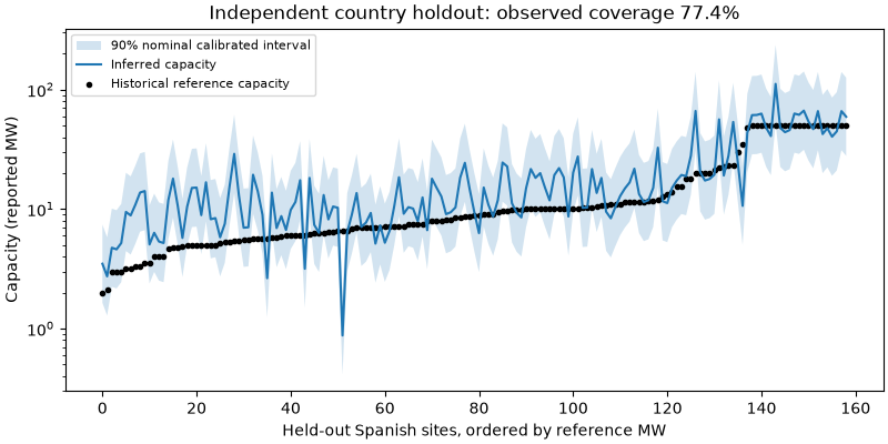
{'n': 159, 'mae_mw': 6.391299581325955, 'rmse_mw': 10.19229115142733, 'r_squared': 0.5349882078849242, 'coverage_nominal': 0.9, 'coverage_observed': 0.7735849056603774}
import hashlib
import json
from pathlib import Path

import matplotlib.pyplot as plt
import numpy as np
import pandas as pd

from orbitalpv.ground_research import evaluate_geometry_capacity, fit_geometry_capacity_model

directory = Path(__file__).resolve().parent if "__file__" in globals() else Path.cwd()
data = directory.parent / "ground_imagery/_data/wiki_solar_join.csv"
provenance = json.loads(data.with_suffix(".csv.meta.json").read_text())
if hashlib.sha256(data.read_bytes()).hexdigest() != provenance["sha256"]:
    raise ValueError("Reference source checksum differs from its recorded provenance")
raw = pd.read_csv(data)
valid = (raw.power > 0) & (raw["panel.area"] > 0) & np.isfinite(raw.power) & raw.GID_0.notna()
frame = raw[valid].assign(
    site_id=lambda f: f.sol_id.astype(str),
    footprint_area_m2=lambda f: f["panel.area"] * 1e6,
    capacity_mw=lambda f: f.power,
)
calibration_countries = ("FRA", "CAN", "ITA")
training = frame[~frame.GID_0.isin((*calibration_countries, "ESP"))]
calibration = frame[frame.GID_0.isin(calibration_countries)]
reference = frame[frame.GID_0 == "ESP"]
model = fit_geometry_capacity_model(
    training,
    calibration,
    capacity_basis="reported",
    area_basis="OSM polygon proxy",
    source="Dunnett2020 Figshare v2 historical Wiki Solar",
    group_column="GID_0",
)
metrics = evaluate_geometry_capacity(model, reference)
prediction = model.predict(reference, area_basis="OSM polygon proxy", allow_extrapolation=True)
prediction["reference_mw"] = reference.capacity_mw.to_numpy()
prediction = prediction.sort_values("reference_mw")

fig, ax = plt.subplots(figsize=(8, 4), constrained_layout=True)
x = np.arange(len(prediction))
ax.fill_between(
    x, prediction.lower_mw, prediction.upper_mw, alpha=0.2, label="90% nominal calibrated interval"
)
ax.plot(x, prediction.capacity_mw, label="Inferred capacity")
ax.scatter(x, prediction.reference_mw, s=9, c="black", label="Historical reference capacity")
ax.set(
    xlabel="Held-out Spanish sites, ordered by reference MW",
    ylabel="Capacity (reported MW)",
    yscale="log",
    title=f"Independent country holdout: observed coverage {metrics['coverage_observed']:.1%}",
)
ax.legend(fontsize=8)
print(
    {
        key: metrics[key]
        for key in ("n", "mae_mw", "rmse_mw", "r_squared", "coverage_nominal", "coverage_observed")
    }
)
plt.show()
Total running time of the script: (0 minutes 0.218 seconds)