Note
Go to the end to download the full example code.
Tower height, tracking and longest darkness#
Compare three illustrative points in NASA PGDA Sites 01, 04 and 11, with 2, 5 and 20 m panel elevations. Fixed arrays are vertical and face true north; tracking is ideal two-axis with no motor consumption or mutual shading. Darkness means <=1% of the solar disc visible, resolved at two-hour steps.
import matplotlib.pyplot as plt
from _lunar_analysis import analysis

from orbitalpv import lunar

summary = analysis.compare_sites()
# The public darkness metric uses interval boundaries and explicit visibility.
p = analysis.profile("01", 5)
print(
    "Site01 longest darkness [h]:",
    lunar.longest_darkness_hours(
        p.time_s,
        (p.terrain_visible_fraction * p.earth_visible_fraction).to_numpy()[:-1],
    ),
)
fig, axes = plt.subplots(1, 2, figsize=(11, 4.5), layout="constrained")
for site, color in [("01", "#c77629"), ("04", "#398c99"), ("11", "#7565a8")]:
    for mode, style in [("sun_tracking", "-"), ("fixed", "--")]:
        values = summary[(summary.site == site) & (summary["mode"] == mode)]
        axes[0].plot(
            values.tower_height_m,
            values.energy_kwh_m2,
            style,
            marker="o",
            color=color,
            label=f"Site {site} · {mode.replace('_', ' ')}",
        )
    values = summary[(summary.site == site) & (summary["mode"] == "sun_tracking")]
    axes[1].plot(
        values.tower_height_m, values.longest_darkness_h, "o-", color=color, label=f"Site {site}"
    )
axes[0].set(
    ylabel="Modelled 2026 DC yield [kWh/m²]", title="Height benefit depends on local terrain"
)
axes[1].set(
    ylabel="Longest modelled darkness [hours]",
    title="More annual energy does not guarantee survival",
)
for ax in axes:
    ax.set_xlabel("Panel height above ground [m]")
    ax.set_xticks([2, 5, 20])
    ax.grid(alpha=0.2)
    ax.legend(fontsize=8)
print(summary.to_string(index=False))
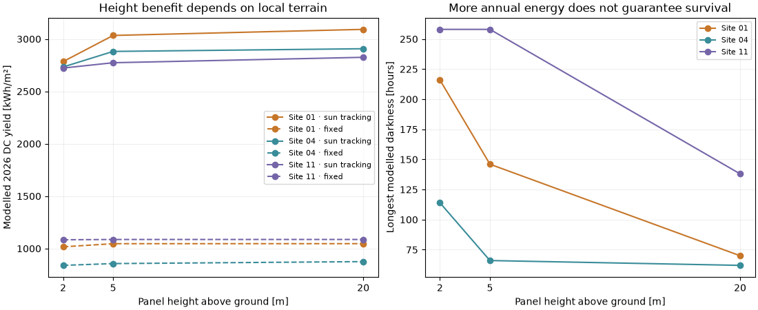
Site01 longest darkness [h]: 146.0
site  tower_height_m         mode  energy_kwh_m2  mean_visible_fraction  longest_darkness_h                                                 model
  01               2        fixed    1016.128041               0.830023               216.0 2026 geometric scenario; constant 25 C cells; 2h step
  01               2 sun_tracking    2784.201679               0.830023               216.0 2026 geometric scenario; constant 25 C cells; 2h step
  01               5        fixed    1046.170658               0.906480               146.0 2026 geometric scenario; constant 25 C cells; 2h step
  01               5 sun_tracking    3033.742236               0.906480               146.0 2026 geometric scenario; constant 25 C cells; 2h step
  01              20        fixed    1046.455542               0.924276                70.0 2026 geometric scenario; constant 25 C cells; 2h step
  01              20 sun_tracking    3091.795292               0.924276                70.0 2026 geometric scenario; constant 25 C cells; 2h step
  04               2        fixed     839.339734               0.814660               114.0 2026 geometric scenario; constant 25 C cells; 2h step
  04               2 sun_tracking    2732.751957               0.814660               114.0 2026 geometric scenario; constant 25 C cells; 2h step
  04               5        fixed     856.291164               0.860269                66.0 2026 geometric scenario; constant 25 C cells; 2h step
  04               5 sun_tracking    2881.282141               0.860269                66.0 2026 geometric scenario; constant 25 C cells; 2h step
  04              20        fixed     875.091733               0.868085                62.0 2026 geometric scenario; constant 25 C cells; 2h step
  04              20 sun_tracking    2906.960007               0.868085                62.0 2026 geometric scenario; constant 25 C cells; 2h step
  11               2        fixed    1083.578145               0.812185               258.0 2026 geometric scenario; constant 25 C cells; 2h step
  11               2 sun_tracking    2722.583563               0.812185               258.0 2026 geometric scenario; constant 25 C cells; 2h step
  11               5        fixed    1086.339724               0.827586               258.0 2026 geometric scenario; constant 25 C cells; 2h step
  11               5 sun_tracking    2773.328209               0.827586               258.0 2026 geometric scenario; constant 25 C cells; 2h step
  11              20        fixed    1086.552942               0.843418               138.0 2026 geometric scenario; constant 25 C cells; 2h step
  11              20 sun_tracking    2825.085388               0.843418               138.0 2026 geometric scenario; constant 25 C cells; 2h step
Compare the best feasible PV/battery candidate at each height, adding an explicitly assumed tower mass of 20 kg + 5 kg/m. This is a design-grid sweep, not a structural analysis or a globally optimal lunar installation.
tradeoff = analysis.tower_tradeoff("01")
fig, ax = plt.subplots(figsize=(7, 4), layout="constrained")
valid = tradeoff[tradeoff.feasible]
ax.bar(
    valid.tower_height_m.astype(str),
    valid.scenario_mass_kg,
    label="PV + battery scenario",
    color="#398c99",
)
ax.bar(
    valid.tower_height_m.astype(str),
    valid.tower_mass_kg,
    bottom=valid.scenario_mass_kg,
    label="Assumed tower",
    color="#c77629",
)
ax.set(
    xlabel="Tower height [m]",
    ylabel="Modelled component mass [kg]",
    title="Site01: lowest feasible mass among tested candidates",
)
ax.legend(fontsize=8)
print(tradeoff.to_string(index=False))
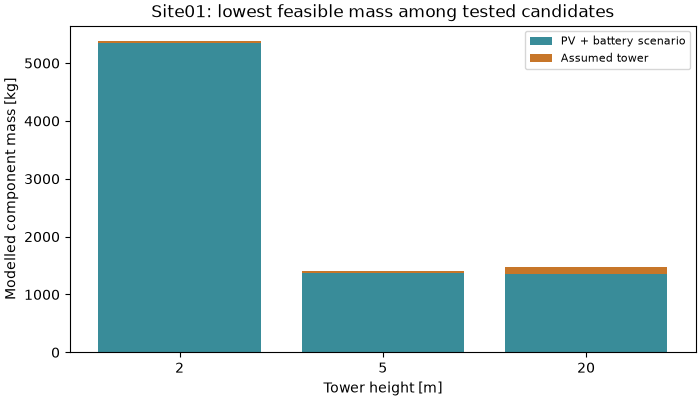
array_area_m2  capacity_wh  unserved_energy_wh  final_soc  minimum_soc  terminal_soc_satisfied  feasible  scenario_mass_kg site  tower_height_m  tower_mass_kg  total_scenario_mass_kg
          6.0     800000.0                 0.0       0.95     0.307168                    True      True       5351.333333   01               2             30             5381.333333
         10.0     200000.0                 0.0       0.95     0.101107                    True      True       1363.333333   01               5             45             1408.333333
          6.0     200000.0                 0.0       0.95     0.224403                    True      True       1351.333333   01              20            120             1471.333333
Numerical sensitivity is material: a coarse azimuth envelope can connect separate shadow events. This comparison is not a confidence interval.
sensitivity = analysis.resolution_sensitivity()
fig, axes = plt.subplots(1, 2, figsize=(9, 3.8), layout="constrained")
for step, values in sensitivity.groupby("timestep_h"):
    degrees = 360 / values.azimuth_bins
    axes[0].plot(degrees, values.july_30day_energy_kwh_m2, "o-", label=f"{step:g} h time step")
    axes[1].plot(degrees, values.longest_darkness_h, "o-", label=f"{step:g} h time step")
axes[0].set(ylabel="July 30-day yield [kWh/m²]", title="Refining the horizon changes yield")
axes[1].set(ylabel="Longest darkness [h]", title="Outage duration needs resolution checks")
for ax in axes:
    ax.set(xlabel="Horizon sector width [degrees]", xticks=[1, 2, 4])
    ax.grid(alpha=0.2)
    ax.legend(fontsize=8)
print(sensitivity.to_string(index=False))
plt.show()
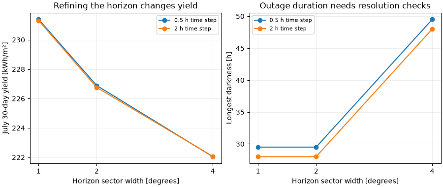
azimuth_bins  timestep_h  july_30day_energy_kwh_m2  longest_darkness_h
          90         2.0                222.066336                48.0
          90         0.5                222.045979                49.5
         180         2.0                226.759887                28.0
         180         0.5                226.891438                29.5
         360         2.0                231.315815                28.0
         360         0.5                231.386435                29.5
Total running time of the script: (0 minutes 4.794 seconds)