Note
Go to the end to download the full example code.
Real MetOp particles and an Earth-view benchmark#
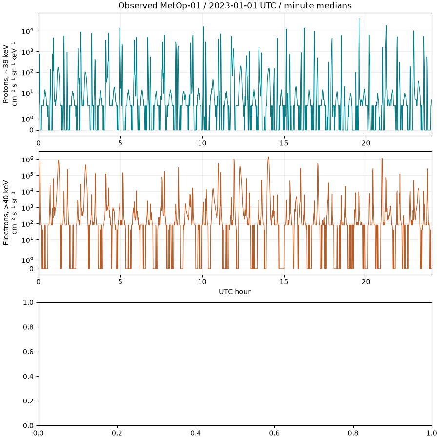
The upper panels use actual 2023-01-01 NOAA MetOp-01 observations, reduced to minute medians. Electron and proton units differ; neither is a solar-cell dose. The final panel is a declared uniform-Earth numerical scenario, not CERES data. All inputs are pinned locally, so this example executes without network access.
import hashlib
import json
from pathlib import Path

import matplotlib.pyplot as plt
import numpy as np
import pandas as pd

import orbitalpv as opv

directory = Path(__file__).resolve().parent if "__file__" in globals() else Path.cwd()
root = next(
    parent for parent in (directory, *directory.parents) if (parent / "pyproject.toml").exists()
)
data = root / "analysis/environmental_inputs/data"
provenance = json.loads((data / "provenance.json").read_text())
path = data / "metop01_20230101_minutes.csv"
if hashlib.sha256(path.read_bytes()).hexdigest() != provenance["snapshot_sha256"]:
    raise ValueError("Observation snapshot checksum failed")
observations = pd.read_csv(path, parse_dates=["minute_utc"])
hours = (observations.minute_utc - observations.minute_utc.iloc[0]).dt.total_seconds() / 3600
Preserve the different energy bins and units in separate axes. Symlog retains measured zeros; a logarithmic plot must not silently erase them.
fig, axes = plt.subplots(3, 1, figsize=(9.0, 9.0), constrained_layout=True)
axes[0].plot(hours, observations.proton_39kev_median_per_cm2_s_sr_kev, color="#007e87", lw=1)
axes[0].set(
    yscale="symlog",
    ylabel="Protons, ~39 keV\ncm⁻² s⁻¹ sr⁻¹ keV⁻¹",
    title="Observed MetOp-01 / 2023-01-01 UTC / minute medians",
)
axes[1].plot(hours, observations.electron_gt40kev_median_per_cm2_s_sr, color="#bc5b24", lw=1)
axes[1].set(yscale="symlog", xlabel="UTC hour", ylabel="Electrons, >40 keV\ncm⁻² s⁻¹ sr⁻¹")
for axis in axes[:2]:
    axis.set_xlim(0, 24)
    axis.grid(alpha=0.2)
The geometric benchmark includes emission angle, panel incidence and inverse distance squared. At nadir the independent uniform-Earth result is F(R/r)^2.
radius = 6_371_008.8
lat_edges, lon_edges = np.linspace(-90, 90, 181), np.linspace(-180, 180, 361)
areas = opv.environment_data.earth_grid_cell_areas(lat_edges, lon_edges)
latitude, longitude = np.meshgrid(
    (lat_edges[1:] + lat_edges[:-1]) / 2, (lon_edges[1:] + lon_edges[:-1]) / 2, indexing="ij"
)
angles = np.arange(0, 181, 15)
values = []
for angle in angles:
    theta = np.deg2rad(angle)
    projected = opv.environment_data.earth_flux_to_panel(
        [radius + 550_000, 0, 0],
        [-np.cos(theta), np.sin(theta), 0],
        latitude,
        longitude,
        np.full(areas.shape, 240.0),
        areas,
    )
    values.append(projected.irradiance_w_m2)
axes[2].plot(angles, values, "o-", color="#35496c", label="Spherical grid integration")
axes[2].scatter(
    [0],
    [240 * (radius / (radius + 550_000)) ** 2],
    marker="x",
    s=100,
    color="#d26031",
    label="Independent nadir analytic reference",
    zorder=5,
)
axes[2].set(
    xlabel="Panel-normal angle from nadir (degrees)",
    ylabel="Earth IR on panel (W/m²)",
    title="Modeled uniform 240 W/m² Earth / altitude 550 km",
)
axes[2].legend(fontsize=9)
axes[2].grid(alpha=0.2)
plt.show()
Total running time of the script: (0 minutes 0.422 seconds)