Note
Go to the end to download the full example code.
Integrate particle spectra before estimating remaining power#
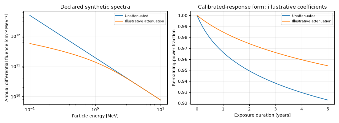
This sensitivity example uses synthetic particle fluence, a synthetic NIEL curve and an explicit empirical response. It illustrates units and the impact of a supplied attenuation curve; it does not calculate a real orbit’s dose.
import matplotlib.pyplot as plt
import numpy as np

from orbitalpv import physics as opv

energy = np.geomspace(0.1, 10, 201)
spectrum = energy**-1.4
spectrum *= 1e12 / np.trapezoid(spectrum, energy)
niel = 0.01 / np.sqrt(energy)
response = opv.RadiationResponse(coefficient=0.08, reference_fluence_cm2=1e12)
years = np.linspace(0, 5, 51)

fig, axes = plt.subplots(1, 2, figsize=(11, 4))
for label, transmission in (
    ("Unattenuated", np.ones_like(energy)),
    ("Illustrative attenuation", 1 - np.exp(-energy / 0.8)),
):
    exposure = opv.radiation_equivalent_fluence(
        energy,
        spectrum,
        niel,
        reference_niel_mev_cm2_g=0.01,
        shielding_transmission=transmission,
    )
    retention = opv.retained_power_fraction(years * exposure.equivalent_fluence_cm2, response)
    axes[0].loglog(energy, spectrum * transmission, label=label)
    axes[1].plot(years, retention, label=label)
axes[0].set(
    xlabel="Particle energy [MeV]",
    ylabel="Annual differential fluence [cm⁻² MeV⁻¹]",
    title="Declared synthetic spectra",
)
axes[1].set(
    xlabel="Exposure duration [years]",
    ylabel="Remaining-power fraction",
    title="Calibrated-response form; illustrative coefficients",
)
for axis in axes:
    axis.grid(alpha=0.25)
    axis.legend(fontsize=8)
fig.tight_layout()
plt.show()
Total running time of the script: (0 minutes 0.280 seconds)