Note
Go to the end to download the full example code.
Mars year: latitude, dust and daily photovoltaic energy#
A horizontal 1-kW reference array at 1361 W/m² and 25°C. Constant tau=0.7, clean panels and fixed cell temperature are scenario assumptions. The map is modelled potential, not a map of measured surface solar resources. It uses the simple Lorenz horizontal approximation, with its diurnal limitations.
import matplotlib.pyplot as plt
import numpy as np

from orbitalpv import PvwattsReference, mars

reference = PvwattsReference(1000, 0.0)
sols = np.linspace(0, 668.6, 50)
latitudes = np.linspace(-90, 90, 25)
dates = 2458449.5 + sols * mars.MARS_SOL_SECONDS / 86400
energy = np.empty((len(latitudes), len(sols)))
for i, latitude in enumerate(latitudes):
    for j, date in enumerate(dates):
        profile = mars.simulate_mars_sol(
            julian_date_tt=float(date),
            latitude_deg=float(latitude),
            reference=reference,
            optical_depth=0.7,
            cell_temperature_c=25,
            samples=145,
        )
        energy[i, j] = profile.attrs["energy_wh"] / 1000
fig, ax = plt.subplots(figsize=(10, 4.8), layout="constrained")
mesh = ax.pcolormesh(sols, latitudes, energy, cmap="magma", shading="auto")
fig.colorbar(mesh, ax=ax, label="kWh/sol per reference kW")
ax.set(
    xlabel="Sols since representative 2018-11-27 date",
    ylabel="Planetographic latitude (°N)",
    title="Mars seasonal PV scenario — constant atmosphere, clean horizontal panels",
)
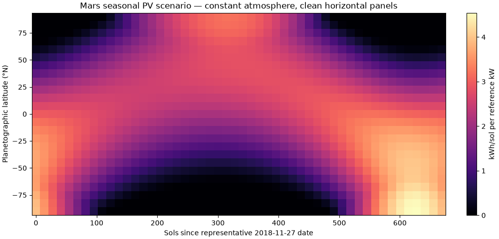
[Text(0.5, 18.503588541666666, 'Sols since representative 2018-11-27 date'), Text(18.503588541666673, 0.5, 'Planetographic latitude (°N)'), Text(0.5, 1.0, 'Mars seasonal PV scenario — constant atmosphere, clean horizontal panels')]
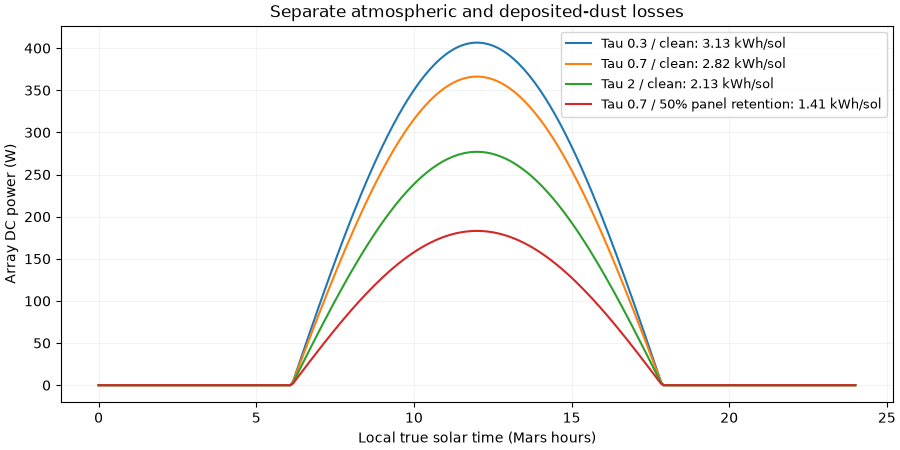
Atmospheric opacity and surface soiling are independent controls.
fig, ax = plt.subplots(figsize=(9, 4.5), layout="constrained")
for tau, dust, label in [
    (0.3, 1, "Tau 0.3 / clean"),
    (0.7, 1, "Tau 0.7 / clean"),
    (2, 1, "Tau 2 / clean"),
    (0.7, 0.5, "Tau 0.7 / 50% panel retention"),
]:
    p = mars.simulate_mars_sol(
        julian_date_tt=2458449.5,
        latitude_deg=4.502,
        reference=reference,
        optical_depth=tau,
        cell_temperature_c=25,
        array_dust_factor=dust,
    )
    ax.plot(p.ltst_h, p.dc_power_w, label=f"{label}: {p.attrs['energy_wh'] / 1000:.2f} kWh/sol")
ax.set(
    xlabel="Local true solar time (Mars hours)",
    ylabel="Array DC power (W)",
    title="Separate atmospheric and deposited-dust losses",
)
ax.legend(fontsize=9)
ax.grid(alpha=0.15)
plt.show()
Total running time of the script: (0 minutes 1.890 seconds)