Note
Go to the end to download the full example code.
Space data centers: orbit, eclipse seasons, and power balance#
Compare orbit choices motivated by published space-computing studies using
the public orbitalpv API. This is an offline design study, with explicit
orbital and electrical assumptions, rather than a flight ephemeris or a
prediction of deployed data-center capacity.
Published concepts and chosen scenarios#
Google’s Suncatcher paper describes a dawn-dusk sun-synchronous concept and illustrates a compact cluster at 650 km. We choose 06:00 ascending mean local solar time for this example; the paper does not specify a numeric crossing time: https://services.google.com/fh/files/misc/suncatcher_paper.pdf.
The completed European ASCEND feasibility study considers 1,400 km sun-synchronous orbits and thirteen 800 kW compute building blocks. Its public architecture page does not specify crossing time. We choose 06:00 ascending as a design sensitivity, not an ASCEND mission parameter: https://ascend-horizon.eu/activities/ and https://cordis.europa.eu/project/id/101082517.
A 650 km, 10:30 descending imaging-style orbit is an analyst-selected control case that isolates the effect of local crossing time. It is not the orbit of a named imaging mission.
Google reported one prototype launch on 1 October 2026. That hardware test is distinct from the proposed computing constellation modeled here: https://blog.google/innovation-and-ai/models-and-research/google-research/project-suncatcher-prototype/.
Sun-synchronous inclination is estimated from first-order J2 precession. The year is idealized: circular Earth motion, 365.2422 days, fixed 23.43928 degree obliquity, and 1 AU Sun distance. The ascending node advances uniformly with the mean Sun; it does not follow the nonuniform physical Sun right ascension. Dates below are days since an idealized March equinox.
The annual sweep uses a cylindrical Earth shadow and point Sun. A separate finite-Sun calculation resolves grazing penumbra. At 1,400 km the point-Sun clearance is very small: a zero cylindrical eclipse duration must not be interpreted as uninterrupted full sunlight.
from __future__ import annotations

import matplotlib.pyplot as plt
import numpy as np

import orbitalpv as opv
Each orbit below uses its own first-order J2 sun-synchronous inclination. Arrays are assumed to track the Sun. We will compare the same electrical design in all three orbits; those ratings are not Google or ASCEND hardware specifications. An 800 kW compute load is motivated by the ASCEND building block, while overhead, array size, temperature, and battery factors are ours.
YEAR_DAYS = 365.2422
OBLIQUITY_RAD = np.deg2rad(23.43928)
scenarios = [
    ("650 km dawn", 650_000.0, 6.0, True, "#0072B2"),
    ("1,400 km dawn", 1_400_000.0, 6.0, True, "#009E73"),
    ("650 km 10:30 descending", 650_000.0, 10.5, False, "#D55E00"),
]
inclinations = [opv.sun_synchronous_inclination_deg(row[1]) for row in scenarios]
periods_s = [opv.circular_orbit_period_s(row[1]) for row in scenarios]
raan_at_equinox = [
    opv.raan_from_local_solar_time_deg(row[2], ascending=row[3]) for row in scenarios
]

fig = plt.figure(figsize=(10, 7), layout="constrained")
ax = fig.add_subplot(111, projection="3d")
longitude = np.linspace(0, 2 * np.pi, 64)
colatitude = np.linspace(0, np.pi, 32)
earth_radius_km = opv.EARTH_EQUATORIAL_RADIUS_M / 1000.0
ax.plot_surface(
    earth_radius_km * np.outer(np.cos(longitude), np.sin(colatitude)),
    earth_radius_km * np.outer(np.sin(longitude), np.sin(colatitude)),
    earth_radius_km * np.outer(np.ones_like(longitude), np.cos(colatitude)),
    color="#c7d8e5",
    alpha=0.25,
    linewidth=0,
)
for scenario, inclination, raan, period in zip(
    scenarios, inclinations, raan_at_equinox, periods_s, strict=True
):
    label, altitude, _, _, color = scenario
    positions = opv.circular_orbit_positions_m(altitude, inclination, raan_deg=raan) / 1000.0
    ax.plot(*positions.T, color=color, label=f"{label}, i={inclination:.2f}°")
    print(f"{label}: first-order inclination={inclination:.6f} deg; period={period / 60:.3f} min")
ax.quiver(0, 0, 0, 10_000, 0, 0, color="#E69F00", linewidth=2, arrow_length_ratio=0.12)
ax.text(10_200, 0, 0, "Sun direction", color="#875900")
ax.set(
    xlabel="Equatorial x [km]",
    ylabel="Equatorial y [km]",
    zlabel="Equatorial z [km]",
    title="Step 1 - Orbit planes at the idealized March equinox",
    xlim=(-11_000, 11_000),
    ylim=(-11_000, 11_000),
    zlim=(-11_000, 11_000),
)
for axis in (ax.xaxis, ax.yaxis, ax.zaxis):
    axis.set_ticks([-8000, 0, 8000])
ax.set_box_aspect((1, 1, 1))
ax.legend(loc="upper left", fontsize=8)
plt.show()
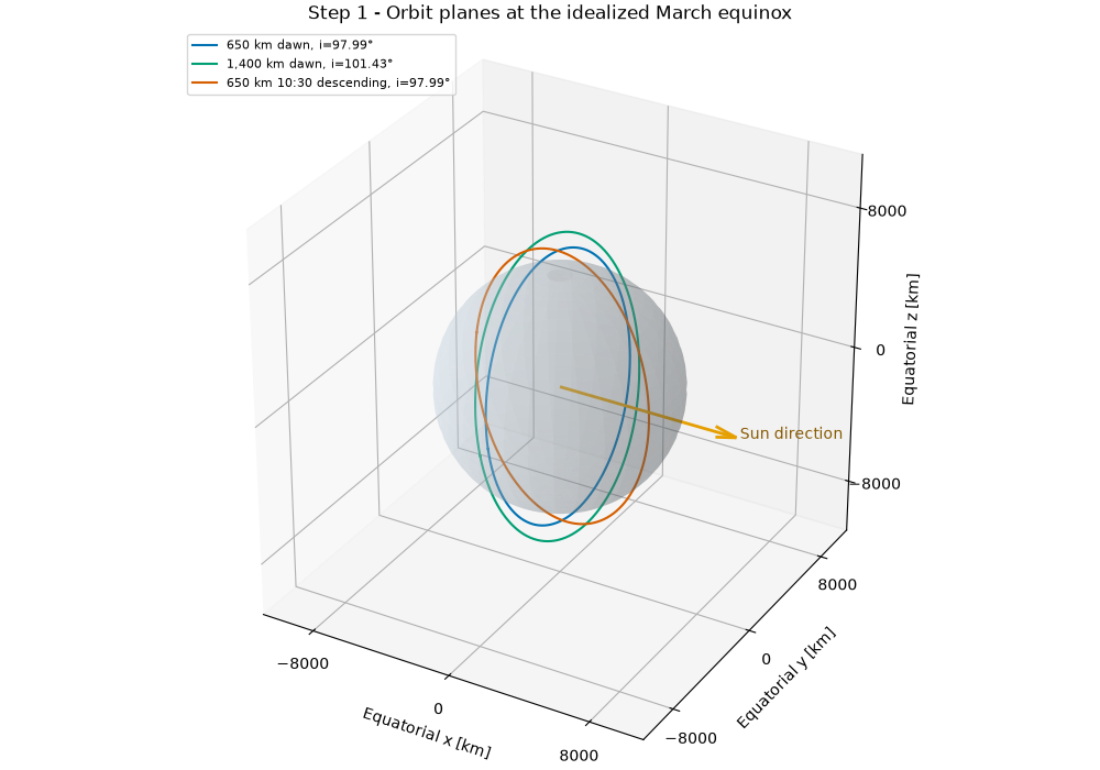
650 km dawn: first-order inclination=97.985997 deg; period=97.728 min
1,400 km dawn: first-order inclination=101.426906 deg; period=113.782 min
650 km 10:30 descending: first-order inclination=97.985997 deg; period=97.728 min
Beta is the angle between the Earth-Sun direction and the orbital plane. Solar declination changes during the year even when the orbit tracks the mean Sun. The annual result is a design approximation, not an operational availability forecast. Four samples per day locate the seasonal minimum beta for the separate finite-Sun check near the 1,400 km point-Sun limit.
days = np.linspace(0, YEAR_DAYS, 1461)
solar_longitude = 2.0 * np.pi * days / YEAR_DAYS
sun_unit = np.column_stack(
    (
        np.cos(solar_longitude),
        np.cos(OBLIQUITY_RAD) * np.sin(solar_longitude),
        np.sin(OBLIQUITY_RAD) * np.sin(solar_longitude),
    )
)
betas = []
worst_indices = []
fig, axes = plt.subplots(3, 1, figsize=(11, 9), sharex=True, layout="constrained")
for scenario, inclination, initial_raan, period in zip(
    scenarios, inclinations, raan_at_equinox, periods_s, strict=True
):
    label, altitude, _, _, color = scenario
    raan = np.deg2rad(initial_raan) + solar_longitude
    inc = np.deg2rad(inclination)
    normal = np.column_stack(
        (np.sin(inc) * np.sin(raan), -np.sin(inc) * np.cos(raan), np.full_like(raan, np.cos(inc)))
    )
    beta = np.rad2deg(np.arcsin(np.clip(np.sum(normal * sun_unit, axis=1), -1, 1)))
    eclipse_s = opv.circular_eclipse_duration_s(altitude, beta)
    sunlit_fraction = 1.0 - eclipse_s / period
    critical = np.rad2deg(
        np.arcsin(opv.EARTH_EQUATORIAL_RADIUS_M / (opv.EARTH_EQUATORIAL_RADIUS_M + altitude))
    )
    betas.append(beta)
    worst_indices.append(int(np.argmin(np.abs(beta))))
    axes[0].plot(days, np.abs(beta), label=label, color=color)
    if label != "650 km 10:30 descending":
        axes[0].axhline(critical, color=color, ls=":", alpha=0.7)
    axes[1].plot(days, eclipse_s / 60.0, color=color)
    axes[2].plot(days, sunlit_fraction * 100.0, color=color)
    annual_sunlit = np.trapezoid(sunlit_fraction, days) / YEAR_DAYS
    print(
        f"{label}: minimum |beta|={np.abs(beta).min():.5f} deg; "
        f"critical={critical:.5f} deg; maximum point-Sun eclipse={eclipse_s.max() / 60:.3f} min; "
        f"annual orbit-averaged sunlight={annual_sunlit:.3%}"
    )
axes[0].set(
    ylabel="Absolute beta [deg]",
    title="Step 2 - Seasonal illumination in a mean-Sun-tracking orbit",
)
axes[0].legend(loc="center", bbox_to_anchor=(0.5, 0.40), ncol=3, fontsize=8)
axes[0].text(
    0.02, 0.30, "Dotted: point-Sun eclipse thresholds", transform=axes[0].transAxes, fontsize=8
)
axes[1].set(
    ylabel="Eclipse per orbit [min]", title="Cylindrical shadow; partial solar occultation excluded"
)
axes[2].set(ylabel="Sunlit fraction [%]", ylim=(55, 102), xlabel="Phase of the idealized year")
axes[2].set_xticks(
    np.linspace(0, YEAR_DAYS, 5),
    [
        "March\nequinox",
        "June\nsolstice",
        "September\nequinox",
        "December\nsolstice",
        "March\nequinox",
    ],
)
for axis in axes:
    axis.set_xlim(0, YEAR_DAYS)
    axis.grid(alpha=0.25)
plt.show()
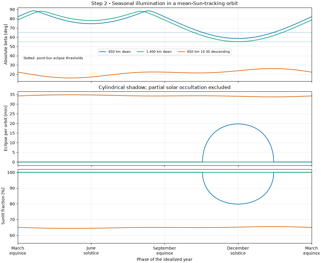
650 km dawn: minimum |beta|=58.57472 deg; critical=65.16412 deg; maximum point-Sun eclipse=19.727 min; annual orbit-averaged sunlight=96.083%
1,400 km dawn: minimum |beta|=55.13381 deg; critical=55.08563 deg; maximum point-Sun eclipse=0.000 min; annual orbit-averaged sunlight=100.000%
650 km 10:30 descending: minimum |beta|=15.91906 deg; critical=65.16412 deg; maximum point-Sun eclipse=34.803 min; annual orbit-averaged sunlight=64.920%
Choose each orbit’s minimum absolute beta, then sample one orbit at 3,601 points. Phase zero is projected solar noon and phase one-half is the center of the shadow passage. The existing Earth/Sun-disc model includes penumbra. It reveals the 1,400 km grazing event hidden by the point-Sun calculation.
phase = np.linspace(0, 1, 3601)
illumination_profiles = []
fig, axes = plt.subplots(2, 1, figsize=(11, 7), layout="constrained")
for scenario, inclination, initial_raan, worst_index, period in zip(
    scenarios, inclinations, raan_at_equinox, worst_indices, periods_s, strict=True
):
    label, altitude, _, _, color = scenario
    raan_deg = initial_raan + np.rad2deg(solar_longitude[worst_index])
    sun_position = opv.ASTRONOMICAL_UNIT_M * sun_unit[worst_index]
    radius = opv.EARTH_EQUATORIAL_RADIUS_M + altitude
    basis = (
        opv.keplerian_orbit_positions_m(
            radius, 0, inclination, raan_deg=raan_deg, true_anomaly_rad=np.array([0, np.pi / 2])
        )
        / radius
    )
    noon_phase = np.arctan2(basis[1] @ sun_position, basis[0] @ sun_position)
    positions = opv.keplerian_orbit_positions_m(
        radius, 0, inclination, raan_deg=raan_deg, true_anomaly_rad=2 * np.pi * phase + noon_phase
    )
    illumination = np.array(
        [opv.earth_occultation_fraction(position, sun_position) for position in positions]
    )
    illumination_profiles.append(illumination)
    axes[0].plot(phase, illumination, color=color, label=label)
    if altitude == 1_400_000.0:
        axes[1].plot((phase - 0.5) * period / 60, illumination, color=color, label="Finite Sun")
    equivalent_dark_s = np.trapezoid(1.0 - illumination, phase * period)
    print(
        f"{label}: finite-Sun minimum illumination={illumination.min():.5f}; "
        f"integrated sunlight loss={equivalent_dark_s / 60:.4f} equivalent dark minutes/orbit"
    )
axes[0].set(
    title="Step 3 - Finite-Sun illumination at each scenario's minimum absolute beta",
    xlabel="Fraction of orbit since projected solar noon",
    ylabel="Visible fraction of solar disc",
    ylim=(-0.03, 1.06),
)
axes[0].legend(fontsize=8, loc="lower left")
axes[1].axhline(1, color="0.45", ls="--", label="Point-Sun approximation")
axes[1].set(
    title="1,400 km dawn detail: partial shadow despite zero point-Sun eclipse",
    xlabel="Minutes from shadow-passage center",
    ylabel="Visible fraction of solar disc",
    xlim=(-5, 5),
    ylim=(0.45, 1.03),
)
axes[1].legend(loc="lower left")
for axis in axes:
    axis.grid(alpha=0.25)
plt.show()
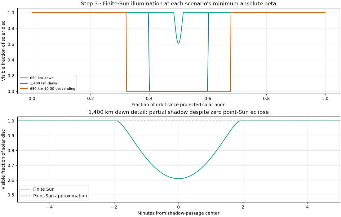
650 km dawn: finite-Sun minimum illumination=0.00000; integrated sunlight loss=19.7293 equivalent dark minutes/orbit
1,400 km dawn: finite-Sun minimum illumination=0.60925; integrated sunlight loss=0.9012 equivalent dark minutes/orbit
650 km 10:30 descending: finite-Sun minimum illumination=0.00000; integrated sunlight loss=34.8044 equivalent dark minutes/orbit
The 800 kW IT load plus an assumed 20% spacecraft overhead needs 960 kW. A 1.5 MW BOL array, 45 degree C cells and 0.96 optical factor are assumed for all three scenarios. Power is modeled with OrbitalPV’s space-calibrated PVWatts reference, not inferred from a proposed spacecraft’s panel area.
Integrate positive surplus and deficit separately. Stored surplus includes charging efficiency; required stored energy includes discharge losses. If the surplus is smaller, adding battery capacity cannot restore a periodic energy balance. The capacity bar is a one-eclipse lower bound with 80% usable depth of discharge. It omits reserve, aging, power limits, thermal behavior, pointing constraints, radiation losses, and all launch or lifecycle costs.
COMPUTE_LOAD_W = 800_000.0
LOAD_W = 1.20 * COMPUTE_LOAD_W
CHARGE_EFFICIENCY = 0.95
DISCHARGE_EFFICIENCY = 0.95
USABLE_DEPTH = 0.80
reference = opv.PvwattsReference(pdc0_w=1_500_000.0, gamma_pdc_per_c=-0.002)
required_kwh = []
recharged_kwh = []
capacity_kwh = []
sustainable = []
for scenario, illumination, period in zip(scenarios, illumination_profiles, periods_s, strict=True):
    irradiance = opv.effective_irradiance_w_m2(
        opv.am0_irradiance(opv.ASTRONOMICAL_UNIT_M),
        illumination,
        np.ones_like(illumination),
        optical_factor=0.96,
    )
    power_w = opv.pvwatts_dc_space(irradiance, 45.0, reference)
    deficit_kwh = float(np.trapezoid(np.maximum(LOAD_W - power_w, 0), phase * period) / 3.6e6)
    surplus_kwh = float(np.trapezoid(np.maximum(power_w - LOAD_W, 0), phase * period) / 3.6e6)
    required = deficit_kwh / DISCHARGE_EFFICIENCY
    recharged = surplus_kwh * CHARGE_EFFICIENCY
    required_kwh.append(required)
    recharged_kwh.append(recharged)
    capacity_kwh.append(required / USABLE_DEPTH)
    sustainable.append(recharged >= required)
    print(
        f"{scenario[0]}: battery-side deficit={required:.2f} kWh; "
        f"available recharge={recharged:.2f} kWh; capacity lower bound={required / USABLE_DEPTH:.2f} kWh; "
        f"cycle energy sufficient={recharged >= required}"
    )

labels = ["650 km\ndawn", "1,400 km\ndawn", "650 km\n10:30 descending"]
x = np.arange(len(labels))
fig, axes = plt.subplots(1, 2, figsize=(12, 5), layout="constrained")
axes[0].bar(x - 0.18, required_kwh, width=0.36, label="Required from storage", color="#D55E00")
axes[0].bar(x + 0.18, recharged_kwh, width=0.36, label="Available to recharge", color="#0072B2")
axes[0].set(
    ylabel="Battery-side energy per worst-case orbit [kWh]",
    title="Step 4 - Can the assumed array replenish the deficit?",
)
axes[0].legend(fontsize=8)
bars = axes[1].bar(x, capacity_kwh, color=[row[4] for row in scenarios])
axes[1].bar_label(bars, fmt="%.1f kWh", padding=4)
axes[1].set(
    ylabel="Nameplate battery energy [kWh]", title="One-eclipse capacity lower bound (80% usable)"
)
axes[1].set_ylim(0, max(capacity_kwh) * 1.3)
for index, feasible in enumerate(sustainable):
    if not feasible:
        axes[1].text(
            index,
            capacity_kwh[index] * 0.45,
            "Array energy\ninsufficient for\nrepeated orbits",
            ha="center",
            color="white",
            fontsize=9,
        )
for axis in axes:
    axis.set_xticks(x, labels)
    axis.grid(axis="y", alpha=0.2)
    axis.set_axisbelow(True)
plt.show()
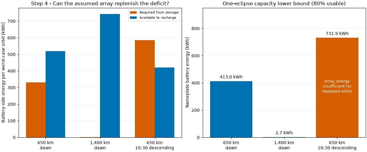
650 km dawn: battery-side deficit=330.41 kWh; available recharge=519.96 kWh; capacity lower bound=413.01 kWh; cycle energy sufficient=True
1,400 km dawn: battery-side deficit=2.14 kWh; available recharge=743.18 kWh; capacity lower bound=2.67 kWh; cycle energy sufficient=True
650 km 10:30 descending: battery-side deficit=585.49 kWh; available recharge=420.22 kWh; capacity lower bound=731.87 kWh; cycle energy sufficient=False
The two dawn cases have different seasonal shadow behavior, and even a small partial shadow can create a load deficit. These are sensitivity results from the stated model. A mission design still needs detailed orbit propagation, attitude, electrical, radiation, thermal, communications and reliability models. In particular, this example does not establish a completed data center’s continuous availability, environmental advantage or commercial feasibility.
Total running time of the script: (0 minutes 1.063 seconds)