Note
Go to the end to download the full example code.
Measured solar spectra from TSIS-1 SIM#
Retrieve three days of real TSIS-1 Spectral Irradiance Monitor (SIM) measurements from LASP LISIRD. Each spectrum resolves the incoming solar irradiance from about 200 to 2400 nm. The published variable wavelength grid and source quality flags remain intact; there is no resampling or gap filling.
These measurements describe the sunlight incident above the atmosphere, not electrical generation. Spectral response or external quantum efficiency measurements for a specific cell would be needed to predict its photocurrent from these spectra.
Source and attribution: TSIS-1 SIM Level-3 daily solar spectral irradiance, LASP/TSIS-1 SIM team, https://lasp.colorado.edu/lisird/data/tsis_ssi_24hr/. See https://lasp.colorado.edu/tsis/data/ for the data description and release notes. This public data product can be recalibrated; cached original responses and checksums identify the exact input used here.
from pathlib import Path
from tempfile import gettempdir

import matplotlib.pyplot as plt

import orbitalpv as opv
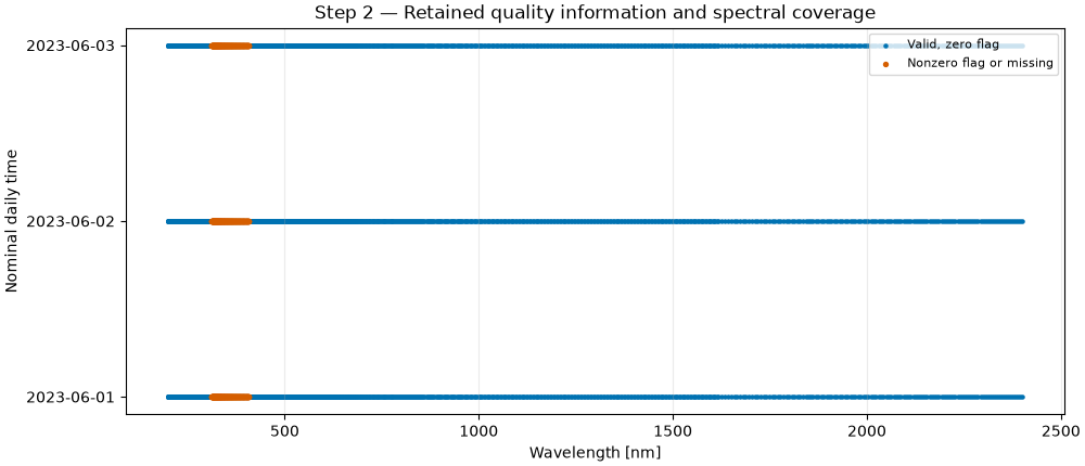
Nominal timestamps represent the centers of daily averaging intervals. The connector returns one row per timestamp and wavelength. Report both counts so thousands of wavelength samples are not mistaken for thousands of independently observed times.
cache = Path(gettempdir()) / "orbitalpv-lisird"
with opv.LisirdConnector() as connector:
    spectrum = connector.spectral_irradiance(
        "tsis_ssi_24hr",
        time_min="2023-06-01",
        time_max="2023-06-04",
        cache_path=cache / "tsis_ssi_2023-06-01.json",
    )

print(
    f"Daily spectra: {spectrum['timestamp'].nunique()}; wavelength observations: {len(spectrum):,}"
)
print(
    f"Wavelength range: {spectrum['wavelength_nm'].min():.3f}-{spectrum['wavelength_nm'].max():.3f} nm"
)
print("Source quality-bit counts:", spectrum["quality_flag"].value_counts(dropna=False).to_dict())
print(f"Raw-response SHA256: {spectrum.attrs['provenance']['sha256']}")

fig, ax = plt.subplots(figsize=(10, 4.8), layout="constrained")
for timestamp, daily in spectrum.groupby("timestamp", sort=True):
    accepted = daily["valid_measurement"] & daily["quality_good"]
    # Keep rejected positions as NaN so the line does not bridge those bins.
    ax.plot(
        daily["wavelength_nm"],
        daily["irradiance_1au_w_m2_nm"].where(accepted),
        linewidth=1,
        label=f"{timestamp:%Y-%m-%d}, zero-flag bins",
    )
flagged = spectrum[spectrum["valid_measurement"] & ~spectrum["quality_good"]]
ax.scatter(
    flagged["wavelength_nm"],
    flagged["irradiance_1au_w_m2_nm"],
    s=3,
    alpha=0.25,
    color="gray",
    label="Nonzero source flags",
)
ax.set(
    xlabel="Wavelength [nm]",
    ylabel="Spectral irradiance at 1 AU [W/m²/nm]",
    title="Step 1 — Three real measured solar spectra",
)
ax.grid(alpha=0.25)
ax.legend(fontsize=8)
plt.show()
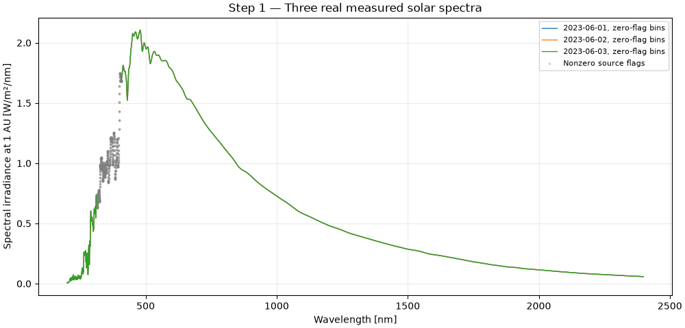
Daily spectra: 3; wavelength observations: 6,312
Wavelength range: 200.015-2399.011 nm
Source quality-bit counts: {0.0: 5274, 4.0: 1038}
Raw-response SHA256: 3ea3fe285f3c66f62a1502efb5bf20328d854ec528a12d6401fc67ee7ba97855
Zero is a conservative selection criterion, not a replacement for the product’s full quality-bit definitions. Nonzero flags remain available to users and may represent caution or additional uncertainty rather than a completely missing observation. No total irradiance is calculated by bridging rejected wavelengths; the measured spectral range also excludes solar energy outside the instrument’s 200-2400 nm coverage.
fig, ax = plt.subplots(figsize=(10, 4.3), layout="constrained")
for row, (_timestamp, daily) in enumerate(spectrum.groupby("timestamp", sort=True)):
    zero = daily["quality_good"] & daily["valid_measurement"]
    ax.scatter(
        daily.loc[zero, "wavelength_nm"],
        [row] * int(zero.sum()),
        s=5,
        color="#0072B2",
        label="Valid, zero flag" if row == 0 else None,
    )
    other = ~zero
    ax.scatter(
        daily.loc[other, "wavelength_nm"],
        [row] * int(other.sum()),
        s=8,
        color="#D55E00",
        label="Nonzero flag or missing" if row == 0 else None,
    )
dates = list(spectrum["timestamp"].drop_duplicates())
ax.set(
    yticks=range(len(dates)),
    yticklabels=[f"{day:%Y-%m-%d}" for day in dates],
    xlabel="Wavelength [nm]",
    ylabel="Nominal daily time",
    title="Step 2 — Retained quality information and spectral coverage",
)
ax.grid(axis="x", alpha=0.25)
ax.legend(fontsize=8)
plt.show()
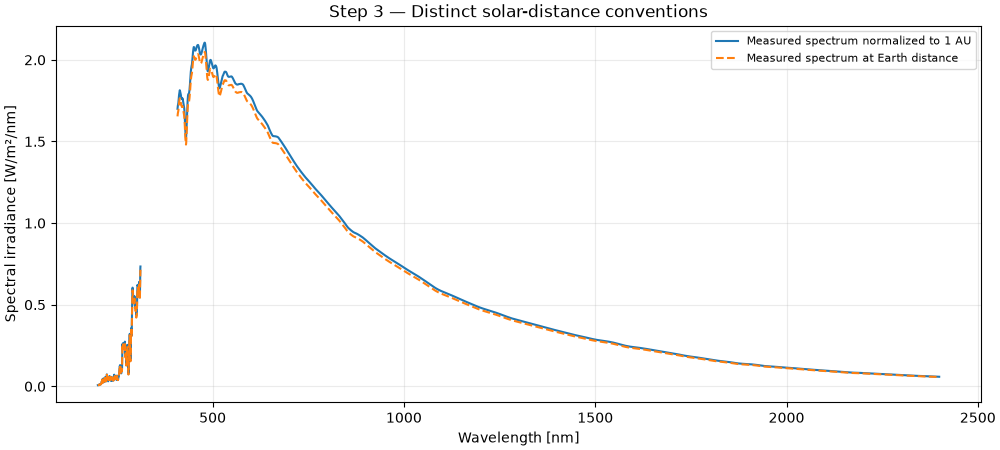
Both are provided by the science product. The ratio illustrates the normalization convention; it is not a cell spectral-response correction. Show only valid, zero-flag bins from the first day and preserve gaps.
first_day = spectrum[spectrum["timestamp"] == spectrum["timestamp"].min()]
accepted = first_day["valid_measurement"] & first_day["quality_good"]
fig, ax = plt.subplots(figsize=(10, 4.5), layout="constrained")
ax.plot(
    first_day["wavelength_nm"],
    first_day["irradiance_1au_w_m2_nm"].where(accepted),
    label="Measured spectrum normalized to 1 AU",
)
ax.plot(
    first_day["wavelength_nm"],
    first_day["irradiance_earth_w_m2_nm"].where(accepted),
    linestyle="--",
    label="Measured spectrum at Earth distance",
)
ax.set(
    xlabel="Wavelength [nm]",
    ylabel="Spectral irradiance [W/m²/nm]",
    title="Step 3 — Distinct solar-distance conventions",
)
ax.grid(alpha=0.25)
ax.legend(fontsize=8)
plt.show()
Total running time of the script: (0 minutes 1.964 seconds)