Note
Go to the end to download the full example code.
Flying Laptop: an empirical reference and its unexplained gap#
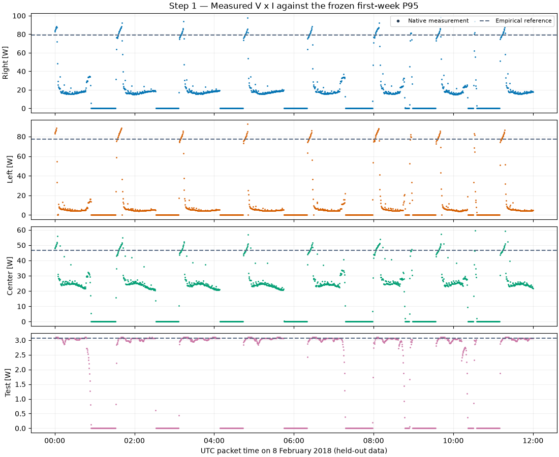
Compare real Flying Laptop array telemetry with a deliberately simple, held-out empirical reference. For each array, freeze the 95th percentile of observed power during 1-7 February 2018, then evaluate 8-28 February without refitting. This is an upper-envelope comparison, not a physical expected-power model. The reference is sample-weighted and depends on what was recorded in the first week; it is neither a rated capacity nor a maximum-power estimate.
The public loss-accounting API keeps the comparison additive and signed. Here, every discrepancy remains unexplained: no orbit, attitude, temperature, maximum-power tracking, load or validated degradation model is supplied. Normal orbital and operational changes can produce large gaps from a constant reference. A positive gap therefore does not establish a recoverable energy loss, efficiency change, degradation or a spacecraft fault. Values above the reference remain visible as negative gaps and surplus.
Source and reproducibility#
FLP Team (2019), FLP Telemetry Data, DaRUS, CC BY 4.0: https://doi.org/10.18419/darus-451.
Official packet definitions and engineering units: https://doi.org/10.18419/darus-456.
February archive: https://darus.uni-stuttgart.de/api/access/datafile/264.
The connector calculates electrical power as calibrated voltage times current
from packet 4900. Timestamps are UTC packet-generation times; the source
allows up to 400 ms of additional acquisition delay. The test channel is
the experimental array aboard the satellite. Signed sensor offsets are kept.
Install pip install "orbital-pv[examples]". The first run downloads the
30 MB monthly archive; subsequent runs reuse the checksum-verified cache used
by the Flying Laptop measurement gallery. No measurements are interpolated or
added. Energy accounting uses trapezoids only between adjacent valid samples
at most 60 seconds apart. This is observed-time accounting under a local
linear approximation, not a full-month energy yield or an inferred duty cycle.
from __future__ import annotations

from pathlib import Path
from tempfile import gettempdir

import matplotlib.dates as mdates
import matplotlib.pyplot as plt
import numpy as np
import pandas as pd
from matplotlib.lines import Line2D
from matplotlib.patches import Patch

import orbitalpv as opv
The fitting window and evaluation window are disjoint UTC intervals. A separate reference is needed for each array because the channels have very different power ranges. The example displays every native observation in the first 12 evaluation hours; markers do not join across missing packets.
MONTH_START = pd.Timestamp("2018-02-01", tz="UTC")
EVALUATION_START = pd.Timestamp("2018-02-08", tz="UTC")
MONTH_STOP = pd.Timestamp("2018-03-01", tz="UTC")
MAX_GAP_S = 60.0
PANELS = ("right", "left", "center", "test")
COLORS = {"right": "#0072B2", "left": "#D55E00", "center": "#009E73", "test": "#CC79A7"}
REFERENCE_COLOR = "#586A83"
GAP_COLOR = "#D55E00"
SURPLUS_COLOR = "#0072B2"

archive = Path(gettempdir()) / "orbitalpv-real-data" / "FLP_TM_HK_2018-02.tar.bz2"
if archive.exists():
    telemetry = opv.load_flying_laptop_power(archive)
else:
    telemetry = opv.fetch_flying_laptop_power("2018-02", archive)

training = telemetry[
    (telemetry["timestamp"] >= MONTH_START) & (telemetry["timestamp"] < EVALUATION_START)
].copy()
evaluation = telemetry[
    (telemetry["timestamp"] >= EVALUATION_START) & (telemetry["timestamp"] < MONTH_STOP)
].copy()
reference_w = training.groupby("panel_id")["power_w"].quantile(0.95)
evaluation["expected_power_w"] = evaluation["panel_id"].map(reference_w)
evaluation["actual_power_w"] = evaluation["power_w"]

reference_table = pd.DataFrame(
    {
        "reference_p95_w": reference_w,
        "training_samples": training.groupby("panel_id").size(),
        "evaluation_samples": evaluation.groupby("panel_id").size(),
    }
).loc[list(PANELS)]
print("Fit: [2018-02-01, 2018-02-08) UTC; evaluation: [2018-02-08, 2018-03-01) UTC")
print(reference_table.to_string(float_format=lambda value: f"{value:.6f}"))
print(f"Source DOI: {telemetry.attrs['dataset_doi']}")
print(f"Archive SHA256: {telemetry.attrs['sha256']}")

detail = evaluation[evaluation["timestamp"] < EVALUATION_START + pd.Timedelta(hours=12)]
fig, axes = plt.subplots(4, 1, figsize=(11, 9), sharex=True, layout="constrained")
for ax, panel_id in zip(axes, PANELS, strict=True):
    panel = detail[detail["panel_id"] == panel_id]
    ax.plot(
        panel["timestamp"],
        panel["actual_power_w"],
        ".",
        ms=2.4,
        color=COLORS[panel_id],
        alpha=0.8,
    )
    ax.axhline(reference_w.loc[panel_id], color=REFERENCE_COLOR, linestyle="--")
    ax.set(ylabel=f"{panel_id.capitalize()} [W]")
    ax.grid(alpha=0.2)
axes[0].set_title("Step 1 — Measured V x I against the frozen first-week P95")
axes[0].legend(
    handles=[
        Line2D([], [], marker=".", linestyle="", color="#243B53", label="Native measurement"),
        Line2D([], [], linestyle="--", color=REFERENCE_COLOR, label="Empirical reference"),
    ],
    loc="upper right",
    ncols=2,
    fontsize=8,
)
axes[-1].set(xlabel="UTC packet time on 8 February 2018 (held-out data)")
axes[-1].xaxis.set_major_locator(mdates.HourLocator(interval=2))
axes[-1].xaxis.set_major_formatter(mdates.DateFormatter("%H:%M"))
plt.show()
Fit: [2018-02-01, 2018-02-08) UTC; evaluation: [2018-02-08, 2018-03-01) UTC
          reference_p95_w  training_samples  evaluation_samples
panel_id
right           78.964078             20043               55054
left            77.556344             20043               55054
center          46.711056             20043               55054
test             3.059895             20043               55054
Source DOI: 10.18419/darus-451
Archive SHA256: 9ec01cfc3128cc4dad522df14cb4aa73191748791a8677e181e4ed4c6e2af1bb
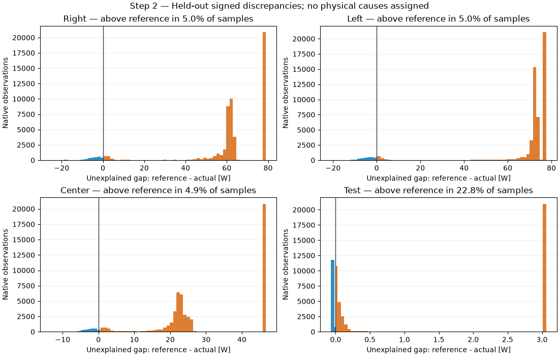
No physical loss stages are supplied. Consequently modeled power equals the empirical reference and the unexplained residual equals reference minus actual power. Negative residuals mean the observation exceeded this reference; they are retained rather than clipped. These histograms are sample counts, not time-weighted estimates of operating-state probabilities.
breakdown = opv.power_loss_breakdown(evaluation, stages=(), group_columns=("panel_id",))
samples = breakdown.samples
fig, axes = plt.subplots(2, 2, figsize=(11, 7), layout="constrained")
for ax, panel_id in zip(axes.flat, PANELS, strict=True):
    panel = samples[(samples["panel_id"] == panel_id) & samples["valid"]]
    gap_w = panel["unexplained_loss_w"].to_numpy(dtype=float)
    edges = np.unique(np.r_[np.linspace(gap_w.min(), gap_w.max(), 66), 0.0])
    counts, edges = np.histogram(gap_w, bins=edges)
    centers = (edges[:-1] + edges[1:]) / 2
    ax.bar(
        centers,
        counts,
        width=np.diff(edges),
        color=np.where(centers < 0, SURPLUS_COLOR, GAP_COLOR),
        alpha=0.8,
    )
    ax.axvline(0, color="#243B53", linewidth=1)
    ax.set(
        title=f"{panel_id.capitalize()} — above reference in {(gap_w < 0).mean():.1%} of samples",
        xlabel="Unexplained gap: reference - actual [W]",
        ylabel="Native observations",
    )
    ax.grid(axis="y", alpha=0.2)
fig.suptitle("Step 2 — Held-out signed discrepancies; no physical causes assigned")
plt.show()
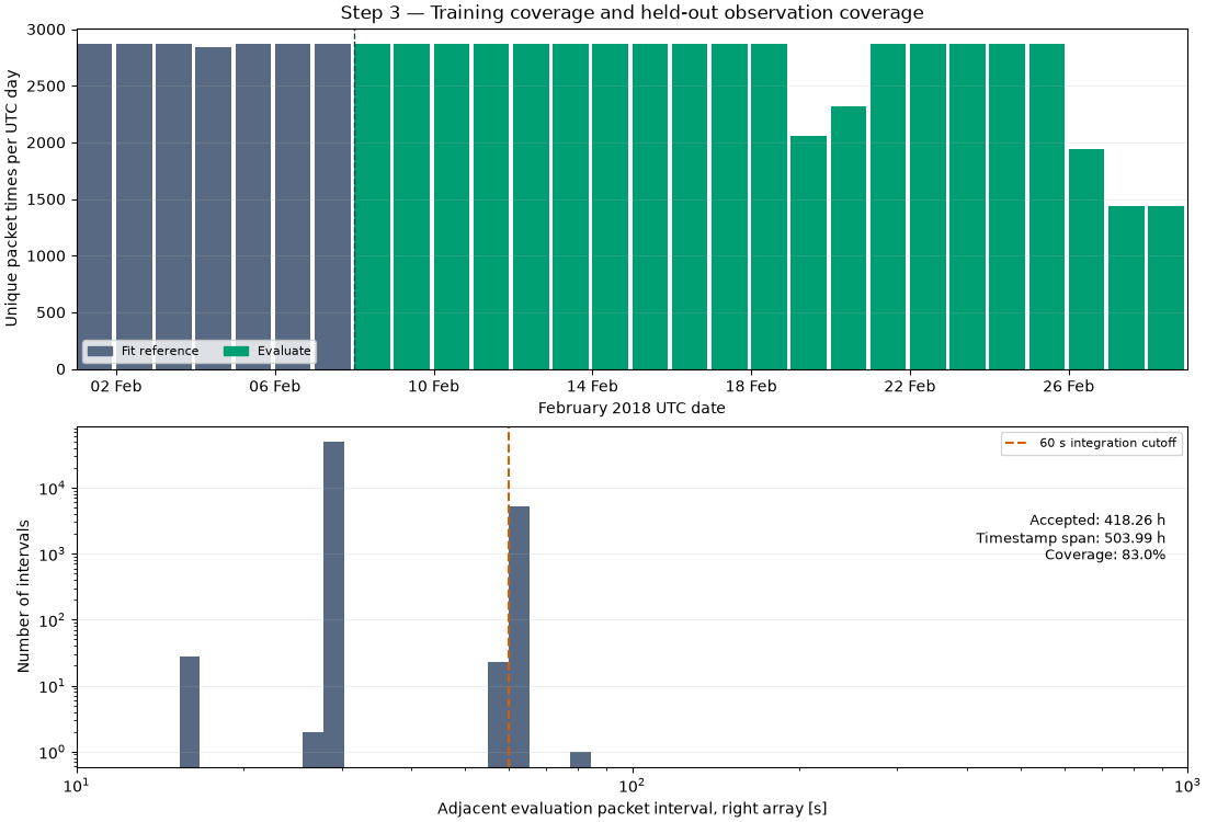
Median native cadence is about 30.15 seconds. The 60-second cutoff conservatively excludes recorded intervals near 60.30 seconds as well as longer gaps; the timing alone does not identify why sampling changed. An interval contributes only when its endpoints are valid and its duration is positive and no greater than this cutoff. No energy is assigned to rejected intervals, and evaluation never bridges the fit split.
Coverage is accepted duration divided by each array’s first-to-last evaluation timestamp span. It is not spacecraft availability. The cadence histogram uses the right array; the summary reports every array separately.
energy = opv.summarize_power_losses(breakdown, max_gap_s=MAX_GAP_S)
totals = energy.totals.set_index("panel_id").loc[list(PANELS)]
print(f"Integration cutoff: {MAX_GAP_S:.0f} s; signed actual power retained")
print(
    totals[
        [
            "observed_duration_h",
            "window_duration_h",
            "coverage_fraction",
            "actual_energy_wh",
            "gap_energy_wh",
            "attributed_energy_wh",
            "unexplained_energy_wh",
            "positive_gap_energy_wh",
            "surplus_energy_wh",
        ]
    ].to_string(float_format=lambda value: f"{value:.6f}")
)

packet_times = telemetry["timestamp"].drop_duplicates().sort_values()
daily_counts = packet_times.groupby(packet_times.dt.floor("D")).size()
right_times = evaluation.loc[evaluation["panel_id"] == "right", "timestamp"].sort_values()
interval_s = right_times.diff().dt.total_seconds().dropna()
print(f"Evaluation cadence: median {interval_s.median():.3f} s; maximum {interval_s.max():.3f} s")

fig, axes = plt.subplots(2, 1, figsize=(11, 7.5), layout="constrained")
axes[0].bar(
    daily_counts.index,
    daily_counts.values,
    width=0.9,
    align="edge",
    color=np.where(daily_counts.index < EVALUATION_START, REFERENCE_COLOR, "#009E73"),
)
axes[0].axvline(EVALUATION_START, color="#243B53", linestyle="--", linewidth=1)
axes[0].set(
    title="Step 3 — Training coverage and held-out observation coverage",
    ylabel="Unique packet times per UTC day",
    xlabel="February 2018 UTC date",
    xlim=(MONTH_START, MONTH_STOP),
)
axes[0].xaxis.set_major_locator(mdates.DayLocator(interval=4))
axes[0].xaxis.set_major_formatter(mdates.DateFormatter("%d %b"))
axes[0].legend(
    handles=[
        Patch(color=REFERENCE_COLOR, label="Fit reference"),
        Patch(color="#009E73", label="Evaluate"),
    ],
    loc="lower left",
    ncols=2,
    fontsize=8,
)
axes[1].hist(interval_s, bins=np.geomspace(10, 1_000, 55), color=REFERENCE_COLOR)
axes[1].axvline(MAX_GAP_S, color=GAP_COLOR, linestyle="--", label="60 s integration cutoff")
axes[1].set(
    xscale="log",
    yscale="log",
    xlabel="Adjacent evaluation packet interval, right array [s]",
    ylabel="Number of intervals",
    xlim=(10, 1_000),
)
axes[1].legend(loc="upper right", fontsize=8)
right_totals = totals.loc["right"]
axes[1].text(
    0.98,
    0.75,
    f"Accepted: {right_totals['observed_duration_h']:.2f} h\n"
    f"Timestamp span: {right_totals['window_duration_h']:.2f} h\n"
    f"Coverage: {right_totals['coverage_fraction']:.1%}",
    transform=axes[1].transAxes,
    ha="right",
    va="top",
    fontsize=9,
)
for ax in axes:
    ax.grid(axis="y", alpha=0.2)
plt.show()
Integration cutoff: 60 s; signed actual power retained
          observed_duration_h  window_duration_h  coverage_fraction  actual_energy_wh  gap_energy_wh  attributed_energy_wh  unexplained_energy_wh  positive_gap_energy_wh  surplus_energy_wh
panel_id
right              418.256446         503.988153           0.829893       7173.980308   25853.254151              0.000000           25853.254151            25946.838006          93.583855
left               418.256446         503.988153           0.829893       4085.354246   28353.086557              0.000000           28353.086557            28433.921143          80.834586
center             418.256446         503.988153           0.829893       7273.937450   12263.262954              0.000000           12263.262954            12313.449647          50.186693
test               418.256446         503.988153           0.829893        774.910318     504.910375              0.000000             504.910375              507.799833           2.889458
Evaluation cadence: median 30.150 s; maximum 79.113 s
A waterfall subtracts below-reference area and adds above-reference area over exactly the same accepted intervals. Both terms are unexplained. The public summary splits intervals at a residual zero crossing, so signed cancellation is explicit. No bars are invented for eclipse, temperature, pointing, degradation or electrical faults without an independently justified model. These kWh describe comparison bookkeeping over observed intervals, not recoverable loss or a full-calendar energy budget.
fig, axes = plt.subplots(2, 2, figsize=(12, 8), layout="constrained")
for ax, panel_id in zip(axes.flat, PANELS, strict=True):
    row = totals.loc[panel_id]
    reference_kwh = float(row["expected_energy_wh"]) / 1_000
    actual_kwh = float(row["actual_energy_wh"]) / 1_000
    below_kwh = float(row["positive_gap_energy_wh"]) / 1_000
    above_kwh = float(row["surplus_energy_wh"]) / 1_000
    after_below = reference_kwh - below_kwh
    heights = [reference_kwh, -below_kwh, above_kwh, actual_kwh]
    bottoms = [0, reference_kwh, after_below, 0]
    ax.bar(
        range(4),
        heights,
        bottom=bottoms,
        width=0.65,
        color=[REFERENCE_COLOR, GAP_COLOR, SURPLUS_COLOR, "#009E73"],
        alpha=0.9,
    )
    for index, level in enumerate([reference_kwh, after_below, actual_kwh]):
        ax.plot([index + 0.325, index + 0.675], [level, level], color="#94A3B8", linewidth=1)
    for index, value in enumerate(heights):
        top = bottoms[index] + max(value, 0)
        label = f"{value:+.3f}" if index in (1, 2) else f"{value:.3f}"
        ax.annotate(
            label, (index, top), xytext=(0, 5), textcoords="offset points", ha="center", fontsize=8
        )
    ax.set(
        title=f"{panel_id.capitalize()} — {row['observed_duration_h']:.2f} observed hours",
        ylabel="Time-integrated comparison [kWh]",
        xticks=range(4),
        xticklabels=[
            "Empirical\nreference",
            "Unexplained\nbelow-reference",
            "Unexplained\nabove-reference",
            "Observed\nV x I",
        ],
        ylim=(0, reference_kwh * 1.18),
    )
    ax.tick_params(axis="x", labelsize=8)
    ax.grid(axis="y", alpha=0.2)
fig.suptitle("Step 4 — Observed-time reconciliation; all discrepancies remain unexplained")
plt.show()
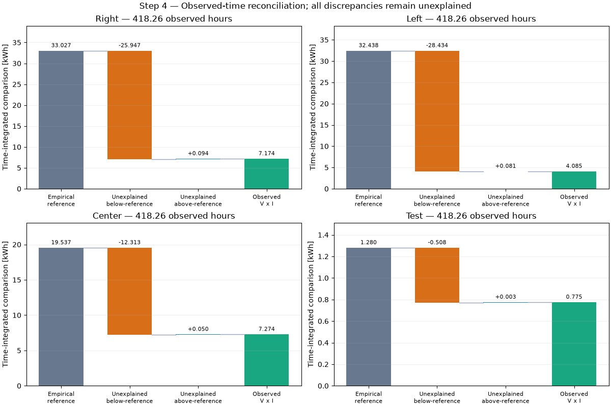
This comparison exposes how large an empirical-reference gap can be even before any physical cause is established. Add independently aligned orbit and attitude, illumination, array temperature, electrical operating state and an appropriate array model before supplying causal loss stages. Keeping their evidence explicit and retaining an unexplained residual is preferable to assigning familiar physical labels to an unsupported reference gap.
Total running time of the script: (0 minutes 9.642 seconds)