Note
Go to the end to download the full example code.
Planning perovskite flight monitoring#
JAXA’s October 30, 2026 update reports bus power delivery on September 10 and plans further I-V monitoring. It publishes no numerical I-V series. This example therefore models a campaign decision, not OrigamiSat-2 performance: can weekly or daily matched sweeps detect a 5% annual loss with 80% probability using a 95% two-sided interval? Noise and drift below are analyst assumptions.
The baseline assumes independent 2% log-power noise. Sensitivities add 3% correlated log noise with a seven-day time scale and bounded ±0.01/year log calibration drift. Daily sweeps consume more acquisition/downlink opportunities; longer monitoring can be more valuable than denser sampling. Only valid, normalized MPP observations count. See the analysis README for the equations, source dates, limitations and reproduction commands.
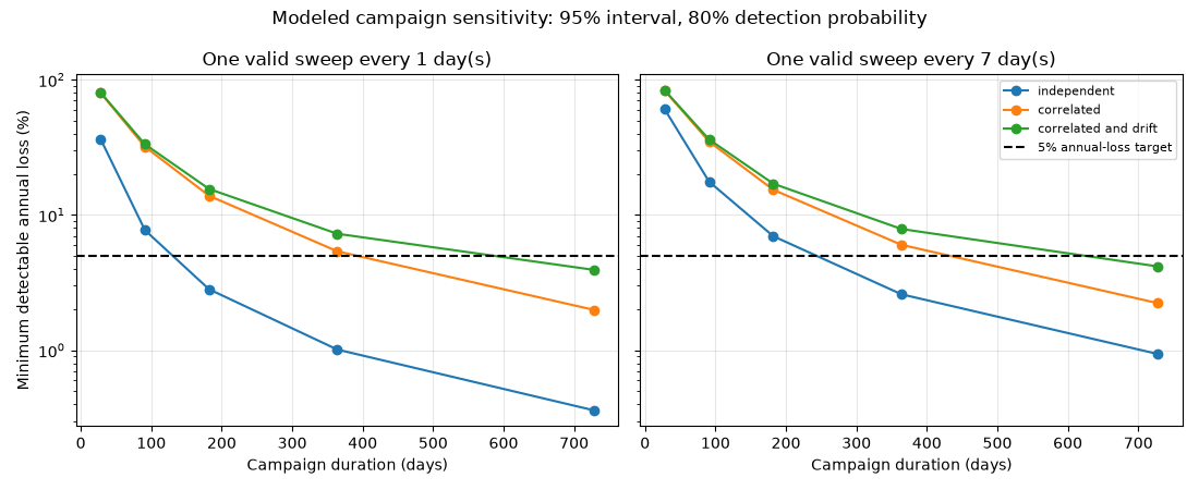
            scenario  cadence_days  observations  duration_days  slope_standard_error_per_year  minimum_detectable_annual_loss  confidence  detection_probability  drift_bound_per_year  detects_five_percent_annual_loss
         independent             1            29           28.0                       0.162133                        0.365063        0.95                    0.8                  0.00                             False
         independent             1            92           91.0                       0.028678                        0.077202        0.95                    0.8                  0.00                             False
         independent             1           183          182.0                       0.010222                        0.028232        0.95                    0.8                  0.00                              True
         independent             1           365          364.0                       0.003629                        0.010115        0.95                    0.8                  0.00                              True
         independent             1           729          728.0                       0.001286                        0.003595        0.95                    0.8                  0.00                              True
         independent             7             5           28.0                       0.330006                        0.603286        0.95                    0.8                  0.00                             False
         independent             7            14           91.0                       0.069188                        0.176207        0.95                    0.8                  0.00                             False
         independent             7            27          182.0                       0.025785                        0.069691        0.95                    0.8                  0.00                             False
         independent             7            53          364.0                       0.009371                        0.025911        0.95                    0.8                  0.00                              True
         independent             7           105          728.0                       0.003360                        0.009369        0.95                    0.8                  0.00                              True
          correlated             1            29           28.0                       0.574983                        0.800285        0.95                    0.8                  0.00                             False
          correlated             1            92           91.0                       0.137543                        0.319779        0.95                    0.8                  0.00                             False
          correlated             1           183          182.0                       0.053288                        0.138682        0.95                    0.8                  0.00                             False
          correlated             1           365          364.0                       0.019774                        0.053891        0.95                    0.8                  0.00                             False
          correlated             1           729          728.0                       0.007167                        0.019879        0.95                    0.8                  0.00                              True
          correlated             7             5           28.0                       0.633525                        0.830495        0.95                    0.8                  0.00                             False
          correlated             7            14           91.0                       0.152962                        0.348538        0.95                    0.8                  0.00                             False
          correlated             7            27          182.0                       0.059513                        0.153572        0.95                    0.8                  0.00                             False
          correlated             7            53          364.0                       0.022143                        0.060150        0.95                    0.8                  0.00                             False
          correlated             7           105          728.0                       0.008038                        0.022267        0.95                    0.8                  0.00                              True
correlated_and_drift             1            29           28.0                       0.574983                        0.804240        0.95                    0.8                  0.01                             False
correlated_and_drift             1            92           91.0                       0.137543                        0.333248        0.95                    0.8                  0.01                             False
correlated_and_drift             1           183          182.0                       0.053288                        0.155738        0.95                    0.8                  0.01                             False
correlated_and_drift             1           365          364.0                       0.019774                        0.072626        0.95                    0.8                  0.01                             False
correlated_and_drift             1           729          728.0                       0.007167                        0.039286        0.95                    0.8                  0.01                              True
correlated_and_drift             7             5           28.0                       0.633525                        0.833852        0.95                    0.8                  0.01                             False
correlated_and_drift             7            14           91.0                       0.152962                        0.361437        0.95                    0.8                  0.01                             False
correlated_and_drift             7            27          182.0                       0.059513                        0.170333        0.95                    0.8                  0.01                             False
correlated_and_drift             7            53          364.0                       0.022143                        0.078761        0.95                    0.8                  0.01                             False
correlated_and_drift             7           105          728.0                       0.008038                        0.041627        0.95                    0.8                  0.01                              True
from dataclasses import asdict
from pathlib import Path

import matplotlib.pyplot as plt
import numpy as np
import pandas as pd

from orbitalpv.analytics import design_degradation_monitoring, log_power_covariance
from orbitalpv.data import load_table


def campaign_table() -> pd.DataFrame:
    """Evaluate 30 duration/cadence/noise combinations from a local input table."""
    directory = Path(__file__).resolve().parent if "__file__" in globals() else Path.cwd()
    cases = load_table(directory / "_data/monitoring_noise_cases.csv")
    rows = []
    for case in cases.to_dict("records"):
        for cadence in (1, 7):
            for duration in (28, 91, 182, 364, 728):
                times = np.arange(0, duration + 1, cadence, dtype=float)
                covariance = log_power_covariance(
                    times,
                    independent_sigma=float(case["independent_sigma"]),
                    correlated_sigma=float(case["correlated_sigma"]),
                    correlation_days=float(case["correlation_days"]),
                )
                design = design_degradation_monitoring(
                    times, covariance, drift_bound_per_year=float(case["drift_bound_per_year"])
                )
                rows.append(
                    {
                        "scenario": case["scenario"],
                        "cadence_days": cadence,
                        **asdict(design),
                        "detects_five_percent_annual_loss": design.minimum_detectable_annual_loss
                        <= 0.05,
                    }
                )
    return pd.DataFrame(rows)


def plot_campaign(results: pd.DataFrame) -> plt.Figure:
    fig, axes = plt.subplots(1, 2, figsize=(11, 4.5), sharey=True)
    for axis, cadence in zip(axes, (1, 7), strict=True):
        subset = results[results.cadence_days == cadence]
        for name, group in subset.groupby("scenario", sort=False):
            axis.plot(
                group.duration_days,
                group.minimum_detectable_annual_loss * 100,
                "o-",
                label=str(name).replace("_", " "),
            )
        axis.axhline(5, color="black", linestyle="--", label="5% annual-loss target")
        axis.set(title=f"One valid sweep every {cadence} day(s)", xlabel="Campaign duration (days)")
        axis.set_yscale("log")
        axis.grid(alpha=0.3)
    axes[0].set_ylabel("Minimum detectable annual loss (%)")
    axes[1].legend(fontsize=8)
    fig.suptitle("Modeled campaign sensitivity: 95% interval, 80% detection probability")
    fig.tight_layout()
    return fig


if __name__ == "__main__":
    results = campaign_table()
    print(results.to_string(index=False))
    plot_campaign(results)
    plt.show()
Total running time of the script: (0 minutes 0.386 seconds)