Ctrl+K

OrbitalPV

  • Satellite PV database
  • User Guide
  • OrbitalPV Example Gallery
  • API Reference
  • Research Library
  • Contributing
  • GitHub
  • Satellite PV database
  • User Guide
  • OrbitalPV Example Gallery
  • API Reference
  • Research Library
  • Contributing
  • GitHub

Section Navigation

  • Real on-orbit data
    • Solar activity: sunlight, X-rays and geomagnetic context
    • Measured GOES proton and electron environment
    • Measured solar spectra from TSIS-1 SIM
    • Free spacecraft research APIs: evidence, archives and geometry
    • Flying Laptop: a month of measured solar-array generation
    • Measured solar irradiance from TSIS-1 and SORCE
    • OPS-SAT photodiodes: real signals and expert annotations
    • Real BIRDS CubeSat solar-panel telemetry
  • PV modelling and loss analytics
    • Flying Laptop: an empirical reference and its unexplained gap
    • Expected versus actual power with known operating states
    • A spacecraft PV loss budget from orbit geometry to converter output
  • Space cell technologies
    • Compare five space solar-cell technologies
    • Temperature and radiation sensitivity of space cells
  • Constellations: imaging, communications, and space computing
    • Starlink Gen1 shell solar generation
    • Sentinel-2 polar imaging and solar-power geometry
    • Compact orbital compute clusters and distributed power
    • GEO weather imagers: surface-irradiance coverage and spacecraft solar power
    • Space data centers: orbit, eclipse seasons, and power balance
  • Orbit Visualization
    • Earth-fixed ground track
    • Representative Earth orbit families
    • Molniya-style highly elliptical orbit
    • Real ISS elements: position, ground track and eclipse
  • Expected PV power versus incidence angle
  • Eclipse fraction along a circular orbit
  • Telemetry-only daily health baseline
  • Constellations: imaging, communications, and space computing
    • Starlink Gen1 shell solar generation
    • Sentinel-2 polar imaging and solar-power geometry
    • Compact orbital compute clusters and distributed power
    • GEO weather imagers: surface-irradiance coverage and spacecraft solar power
    • Space data centers: orbit, eclipse seasons, and power balance
  • Satellite and component database
    • Space-power components and installation evidence
    • Satellite PV evidence coverage
  • Environmental data and Earth-view geometry
    • Real MetOp particles and an Earth-view benchmark
  • Flight calibration, energy budgets and uncertainty
    • Healthy reference calibration with an explicit Gaussian posterior
    • BUPT-1 measured electrical energy budget
    • Real flight power forecasts and coherent uncertainty
  • Ground satellite imagery
    • Ground imagery and mapped solar-farm inputs
    • Rinconada solar plant near Rengo, Chile
    • PV mapping in fewer lines: Icor, Tenerife
    • Detect PV footprints in an unseen satellite image
    • Group mapped PV farms and test an area-capacity model
  • Ground PV research methods
    • Classical cloud optical-flow nowcast
    • Geographic holdout on real Sentinel-2 imagery
    • Construction history as observation brackets
    • Independent capacity calibration and country holdout
  • Lunar surface power and survival
    • Lunar inputs: measurements, computed geometry and NASA references
    • Measured lunar terrain to a local PV yield map
    • Rover routing with terrain, sunlight and battery reserve
    • PV and battery sizing for a continuous lunar load
    • Diviner ground temperatures and a vacuum panel thermal model
    • Tower height, tracking and longest darkness
  • Mars surface photovoltaic performance
    • Mars year: latitude, dust and daily photovoltaic energy
    • InSight: observed energy, atmospheric dust and panel soiling
  • Orbit Visualization
    • Earth-fixed ground track
    • Representative Earth orbit families
    • Molniya-style highly elliptical orbit
    • Real ISS elements: position, ground track and eclipse
  • PV modelling and loss analytics
    • Flying Laptop: an empirical reference and its unexplained gap
    • Expected versus actual power with known operating states
    • A spacecraft PV loss budget from orbit geometry to converter output
  • Real on-orbit data
    • Solar activity: sunlight, X-rays and geomagnetic context
    • Measured GOES proton and electron environment
    • Measured solar spectra from TSIS-1 SIM
    • Free spacecraft research APIs: evidence, archives and geometry
    • Flying Laptop: a month of measured solar-array generation
    • Measured solar irradiance from TSIS-1 and SORCE
    • OPS-SAT photodiodes: real signals and expert annotations
    • Real BIRDS CubeSat solar-panel telemetry
  • Research physics and power systems
    • Integrate particle spectra before estimating remaining power
    • Distinguish mismatch, bypass and open-string I-V signatures
    • Find the current-limiting subcell in a tandem
    • Follow panel temperature through sunlight and eclipse
    • Schedule computing around sunlight and battery limits
  • Space PV business decisions
    • How much customer power can a lunar utility commit?
    • Planning solar-array deployment evidence
    • Lunar DC cable voltage and mass trade
    • When is a tandem array worth its price premium?
    • Space solar delivery versus firm power
    • Repaired panel power: accept or measure again?
    • Planning perovskite flight monitoring
    • Does more solar power unlock continuous payload capacity?
    • Solar-powered AI clusters: links, formation, radiation and cost
    • SpaceX Starmind: from HJT solar cells to usable orbital compute
    • Mars orbital solar-array pointing reserve
  • Space cell technologies
    • Compare five space solar-cell technologies
    • Temperature and radiation sensitivity of space cells
  • OrbitalPV Example Gallery
  • Constellations: imaging, communications, and space computing
  • Starlink Gen1 shell solar generation

Note

Go to the end to download the full example code.

Starlink Gen1 shell solar generation#

Simulate a constellation-scale solar-power profile using only the public orbitalpv API.

The orbital layout follows the FCC-authorized first-generation Starlink 550 km shell: 1,584 satellites, 53° inclination, 72 planes, and 22 satellites per plane.

The electrical assumptions below are illustrative:

  • 3 kW BOL DC reference power per spacecraft;

  • sun-tracking arrays with cosine(AOI) = 1 while illuminated;

  • optical factor = 0.96;

  • fixed 45 °C cell temperature.

These power assumptions are not SpaceX hardware specifications. Change them to study other spacecraft designs.

from __future__ import annotations

import matplotlib.pyplot as plt
import numpy as np

import orbitalpv as opv

SATELLITES = 1_584
PLANES = 72
SATELLITES_PER_PLANE = 22
ALTITUDE_M = 550_000.0
INCLINATION_DEG = 53.0
TIME_SAMPLES = 72

PDC0_PER_SATELLITE_W = 3_000.0
CELL_TEMPERATURE_C = 45.0
OPTICAL_FACTOR = 0.96


def constellation_positions_m(orbit_angle_rad: float) -> np.ndarray:
    """Return one constellation snapshot in a simple ECI frame."""
    radius_m = opv.EARTH_EQUATORIAL_RADIUS_M + ALTITUDE_M
    snapshots: list[np.ndarray] = []

    for plane in range(PLANES):
        raan_deg = plane * 360.0 / PLANES
        phase_offset = 2.0 * np.pi * plane / (PLANES * SATELLITES_PER_PLANE)
        satellite_phase = (
            2.0 * np.pi * np.arange(SATELLITES_PER_PLANE) / SATELLITES_PER_PLANE
            + phase_offset
            + orbit_angle_rad
        )
        snapshots.append(
            opv.keplerian_orbit_positions_m(
                radius_m,
                0.0,
                INCLINATION_DEG,
                raan_deg=raan_deg,
                true_anomaly_rad=satellite_phase,
            )
        )

    positions = np.vstack(snapshots)
    if len(positions) != SATELLITES:
        raise RuntimeError("Unexpected constellation size")
    return positions


radius_m = opv.EARTH_EQUATORIAL_RADIUS_M + ALTITUDE_M
period_s = 2.0 * np.pi * np.sqrt(radius_m**3 / opv.EARTH_STANDARD_GRAVITATIONAL_PARAMETER_M3_S2)
time_s = np.linspace(0.0, period_s, TIME_SAMPLES)
orbit_angle_rad = 2.0 * np.pi * time_s / period_s

sun_position_m = np.array([opv.ASTRONOMICAL_UNIT_M, 0.0, 0.0])
g_am0_w_m2 = opv.am0_irradiance(opv.ASTRONOMICAL_UNIT_M)
reference = opv.PvwattsReference(
    pdc0_w=PDC0_PER_SATELLITE_W,
    gamma_pdc_per_c=-0.002,
)

fleet_power_w: list[float] = []
mean_illumination: list[float] = []
eclipsed_satellites: list[int] = []

for angle in orbit_angle_rad:
    positions_m = constellation_positions_m(float(angle))
    illumination = np.array(
        [opv.earth_occultation_fraction(position_m, sun_position_m) for position_m in positions_m]
    )

    effective_irradiance = opv.effective_irradiance_w_m2(
        g_am0_w_m2,
        illumination,
        np.ones_like(illumination),
        optical_factor=OPTICAL_FACTOR,
    )
    satellite_power_w = opv.pvwatts_dc_space(
        effective_irradiance,
        CELL_TEMPERATURE_C,
        reference,
    )

    fleet_power_w.append(float(np.sum(satellite_power_w)))
    mean_illumination.append(float(np.mean(illumination)))
    eclipsed_satellites.append(int(np.sum(illumination < 0.01)))

fleet_power_w_array = np.asarray(fleet_power_w)
fleet_power_mw = fleet_power_w_array / 1e6
energy_per_orbit_mwh = float(np.trapezoid(fleet_power_w_array, time_s) / 3.6e9)
mean_fleet_power_mw = float(np.mean(fleet_power_mw))

print(f"satellites={SATELLITES}")
print(f"orbital_period_min={period_s / 60.0:.2f}")
print(f"mean_fleet_power_mw={mean_fleet_power_mw:.2f}")
print(f"energy_per_orbit_mwh={energy_per_orbit_mwh:.2f}")
print(f"max_eclipsed_satellites={max(eclipsed_satellites)}")
satellites=1584
orbital_period_min=95.65
mean_fleet_power_mw=2.92
energy_per_orbit_mwh=4.65
max_eclipsed_satellites=529
snapshot_m = constellation_positions_m(0.0)
snapshot_km = snapshot_m / 1000.0
illumination_snapshot = np.array(
    [opv.earth_occultation_fraction(position_m, sun_position_m) for position_m in snapshot_m]
)

fig = plt.figure(figsize=(9, 8))
ax = fig.add_subplot(111, projection="3d")

earth_radius_km = opv.EARTH_EQUATORIAL_RADIUS_M / 1000.0
u = np.linspace(0.0, 2.0 * np.pi, 72)
v = np.linspace(0.0, np.pi, 36)
x = earth_radius_km * np.outer(np.cos(u), np.sin(v))
y = earth_radius_km * np.outer(np.sin(u), np.sin(v))
z = earth_radius_km * np.outer(np.ones_like(u), np.cos(v))
ax.plot_surface(x, y, z, alpha=0.18, linewidth=0)

sunlit = illumination_snapshot >= 0.01
ax.scatter(
    snapshot_km[sunlit, 0],
    snapshot_km[sunlit, 1],
    snapshot_km[sunlit, 2],
    s=5,
    label="Sunlit spacecraft",
)
ax.scatter(
    snapshot_km[~sunlit, 0],
    snapshot_km[~sunlit, 1],
    snapshot_km[~sunlit, 2],
    s=5,
    label="Eclipsed spacecraft",
)

limit_km = (radius_m / 1000.0) * 1.08
ax.set_xlim(-limit_km, limit_km)
ax.set_ylim(-limit_km, limit_km)
ax.set_zlim(-limit_km, limit_km)
ax.set_box_aspect((1, 1, 1))
ax.set(xlabel="ECI x [km]", ylabel="ECI y [km]", zlabel="ECI z [km]")
ax.set_title("Illustrative Starlink Gen1 550 km shell")
ax.legend()
plt.show()
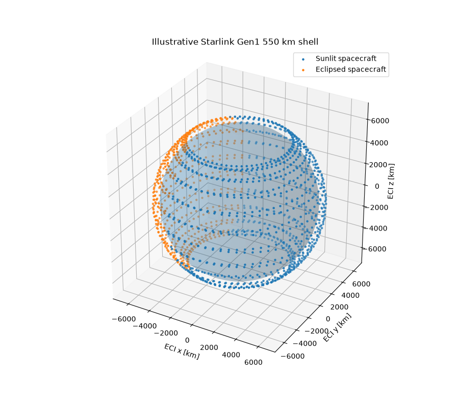
Illustrative Starlink Gen1 550 km shell
fig, ax = plt.subplots(figsize=(9, 4.8))
ax.plot(time_s / 60.0, fleet_power_mw)
ax.set(xlabel="Elapsed time [min]", ylabel="Fleet DC power [MW]")
ax.set_title("Constellation solar generation over one orbital period")
ax.grid(True, alpha=0.3)
plt.show()
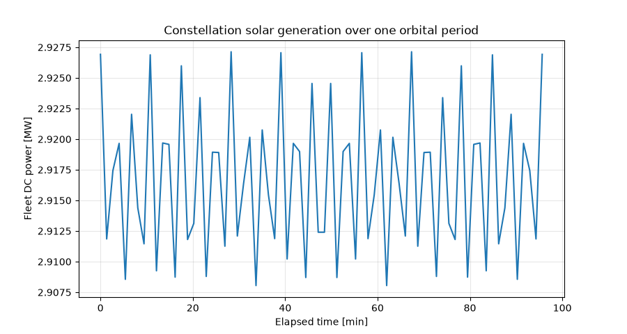
Constellation solar generation over one orbital period

Total running time of the script: (0 minutes 2.593 seconds)

Download Jupyter notebook: plot_starlink_gen1_solar_generation.ipynb

Download Python source code: plot_starlink_gen1_solar_generation.py

Download zipped: plot_starlink_gen1_solar_generation.zip

Gallery generated by Sphinx-Gallery

Edit on GitHub

© Copyright 2026, ASVA Consulting TFE SL.

Created using Sphinx 9.2.0.

Built with the PyData Sphinx Theme 0.23.0.