OrbitalPV Example Gallery#
These examples are executable documentation. They use the same public API that users receive from PyPI:
pip install orbital-pv import orbitalpv as opv
Sphinx-Gallery executes the examples when the documentation site is built. Examples remain deterministic and offline unless a page explicitly documents a live external data source.
Featured sub-galleries#
The real-data gallery retrieves and analyzes measured on-orbit spacecraft PV telemetry. The PV-analytics gallery explains expected-versus-actual power gaps, physical and operational loss categories, and observed-time energy budgets. The space-cell gallery compares silicon, GaAs, 3J, 4J and IMM technologies, including temperature and radiation sensitivity. The constellation gallery includes communications, Earth-imaging and proposed space data-center scenarios. The orbit-visualization gallery contains representative orbit families, ground tracks, and highly elliptical orbit examples.
Constellations: imaging, communications, and space computing#
Use the public orbitalpv API to inspect constellation geometry, sunlight,
and illustrative spacecraft solar generation. The Earth-observation examples
use published nominal mission geometry. The data-center examples investigate
published concepts and explicitly chosen design scenarios.
Example |
What it demonstrates |
|---|---|
GEO weather imagers: surface-irradiance coverage and spacecraft solar power |
GOES, Meteosat, and Himawari viewing geometry, overlap, and eclipse seasons. |
Sentinel-2B/2C design orbits, ground tracks, daylight, and onboard solar power. |
|
Space data centers: orbit, eclipse seasons, and power balance |
Suncatcher- and ASCEND-motivated orbit scenarios, seasonal illumination, finite-Sun penumbra, and an explicit load/storage budget. |
Correlated eclipses in a compact compute cluster versus a hypothetical dispersed ring, including each node’s local power deficit. |
|
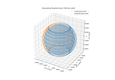
Fleet solar generation for an illustrative Starlink Gen1 shell. |
Install plotting support with pip install "orbital-pv[examples]>=0.6.0".
All five examples run offline, without TLE downloads or additional GIS packages.
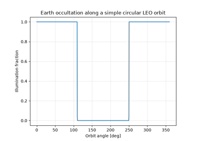
The imagery examples distinguish reflected radiance and retrieved surface irradiance from the spacecraft’s own incoming sunlight and electrical power. Geometric visibility does not guarantee an available image or a valid irradiance retrieval. The data-center studies distinguish proposed constellation layouts from flown hardware and test seasonal shadow instead of assuming constant Sun.
The Starlink example uses the FCC-authorized first-generation 550 km shell geometry: 1,584 satellites at 53° inclination in 72 planes with 22 satellites per plane.
Power-system assumptions throughout the gallery are stated explicitly and are not manufacturer specifications. Arithmetic fleet power is not electrical power sharing between satellites. Each page provides its primary references, time/frame conventions, modelling assumptions, and step-by-step plots.
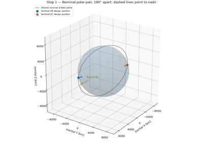
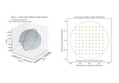
Compact orbital compute clusters and distributed power
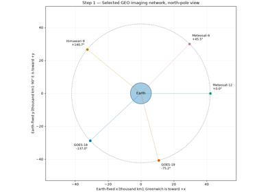
GEO weather imagers: surface-irradiance coverage and spacecraft solar power
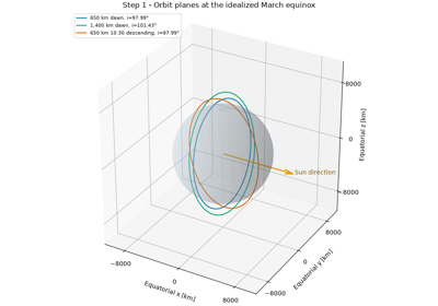
Space data centers: orbit, eclipse seasons, and power balance
Satellite and component database#
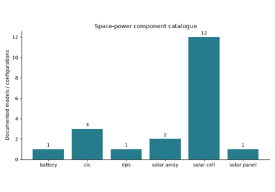
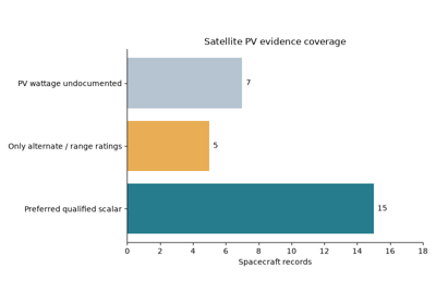
Offline queries, coverage and spacecraft-to-component evidence using the catalogue installed with OrbitalPV. Ratings retain reference conditions and are not live output.
Environmental data and Earth-view geometry#
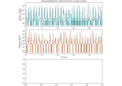
Inspect real NOAA MetOp particle observations and verify a spherical Lambertian Earth-view integrator against an independent analytic reference. Particle measurements and modeled thermal forcing retain their distinct units and measurement boundaries.
See Environmental inputs and attitude for NASA CERES, POES/MetOp, SPENVIS exports, historical orbital elements and SPICE attitude.
Flight calibration, energy budgets and uncertainty#
Research baselines connect measured operating V/I with chronological forecasts, coherent power intervals and electrical-boundary accounting. The Flying Laptop example executes offline on attributed CC BY 4.0 native measurements. The BUPT-1 example displays explicitly precomputed measured aggregates; its raw archive is downloaded only by the corresponding opt-in analysis.
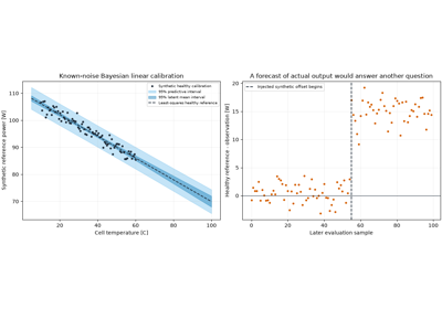
Healthy reference calibration with an explicit Gaussian posterior
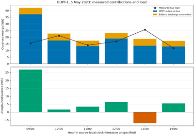
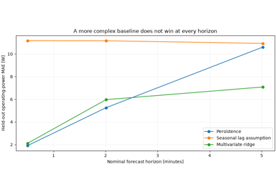
Real flight power forecasts and coherent uncertainty
Ground satellite imagery#
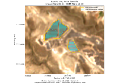
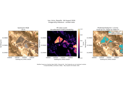
Retrieve ground imagery and mapped renewable-energy features through Python. The walkthroughs cover Cestas in France, Rinconada near Rengo in Chile, and Icor in Tenerife, using the same compact PV mapping utilities. They retain real Sentinel-2 pixels, native quality information, and raw OpenStreetMap inputs related to Dunnett et al. (2020). Each site uses verified local snapshots for offline reproduction.
The image-detection example trains on Cestas and predicts Tenerife and Chile from multispectral pixels. It reports held-out weak-reference errors openly. The inventory example groups mapped features, samples historical GHSL classes, and tests a capacity model against independent records from a withheld country.
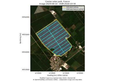
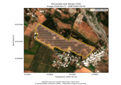
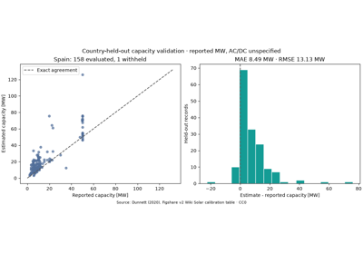
Group mapped PV farms and test an area-capacity model
Ground PV research methods#
Compare geographically held-out mapping, infer geometry with calibrated capacity intervals, match dated footprints, and test cloud-motion nowcasts. Examples say explicitly which inputs are real cached observations and which are synthetic algorithm scenarios. All calls use the public orbitalpv API.
Install orbital-pv[ground-research,examples]. Native spectral assets and
their scale/offset metadata are unchanged; 20 m SWIR resampling creates no
new spatial observations. Optional gated model checkpoints and authenticated
weather products are never downloaded by the gallery.
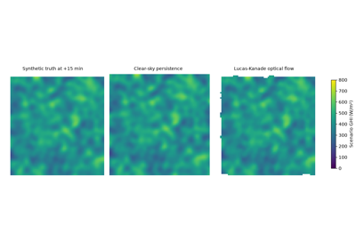

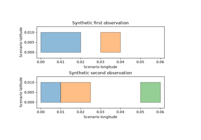
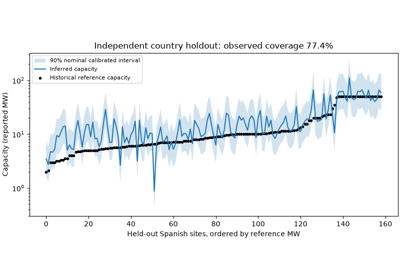
Independent capacity calibration and country holdout
Lunar surface power and survival#
Measured/interpolated LOLA terrain, measured Diviner temperature bins and computed DE421 Sun/Earth geometry drive five reproducible engineering examples. Bundled inputs make every example runnable offline; original downloads and subset provenance can be regenerated with the companion analysis script.
The power, hardware, heater and rover results are model scenarios, not measured lunar PV output or flight-qualified designs. See the lunar modelling guide.
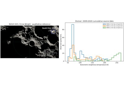
Lunar inputs: measurements, computed geometry and NASA references
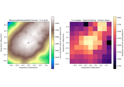
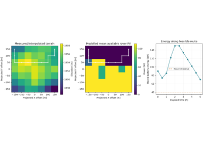
Rover routing with terrain, sunlight and battery reserve
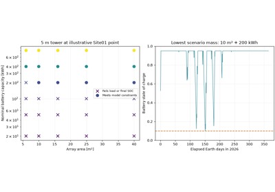
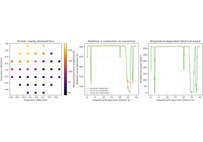
Diviner ground temperatures and a vacuum panel thermal model
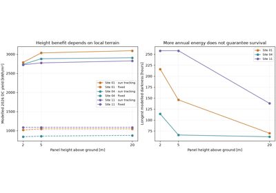
Mars surface photovoltaic performance#
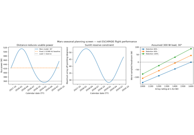
Measured InSight energy and currents, camera-derived opacity, and explicit Mars surface PV scenarios. The examples execute offline on attributed, checksum-pinned observations. Model curves are estimates, not measurements.
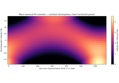
Mars year: latitude, dust and daily photovoltaic energy
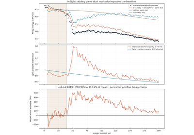
InSight: observed energy, atmospheric dust and panel soiling
Orbit Visualization#
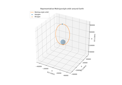
These examples visualize representative Earth-orbit geometries around a 3D planet and as Earth-fixed ground tracks.
They are intentionally deterministic and offline so the documentation build does not depend on live orbital-element services.
The examples are educational geometry visualizations. Production mission analysis should use the OrbitalPV propagation adapters with a traceable OMM, TLE, ephemeris, or SPICE source.
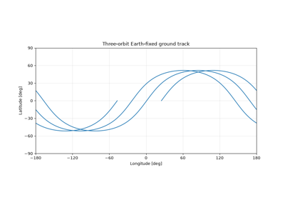
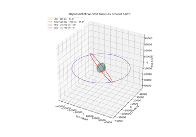
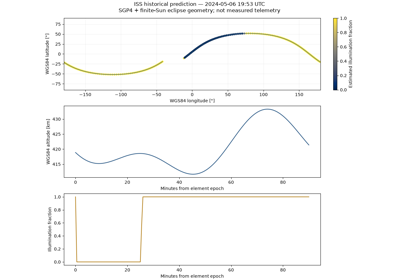
Real ISS elements: position, ground track and eclipse
PV modelling and loss analytics#
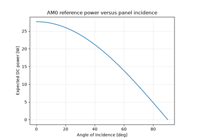
Explain the gap between a declared expected power and actual power, then integrate the same comparison into an energy budget. Named stages retain their evidence and combine into physical or operational categories. The unexplained remainder and any gains remain visible.
Choose the baseline for the question#
Walkthrough |
Expected baseline |
What the breakdown means |
|---|---|---|
Beginning-of-life reference power at a declared irradiance and temperature |
A synthetic design budget through eclipse, pointing, optics, temperature, degradation, wiring, conversion and controller stages |
|
Healthy operating power, with normal geometry and temperature already included |
A synthetic two-array diagnostic example with supported incremental causes, an unexplained remainder, gains and missing observations |
|
A first-week empirical power envelope, evaluated on subsequent measurements |
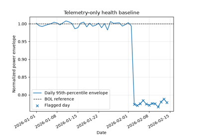
Real voltage/current telemetry with all unsupported causes kept unexplained; this is not an estimate of recoverable energy or physical degradation |
The first two examples run offline and label their simulated observations and assumed parameters explicitly. Flying Laptop reuses the measured-data connector and its cached February 2018 archive; the first run downloads about 30 MB.
Install pip install -U "orbital-pv[examples]>=0.7.0". Each walkthrough includes
four figures and uses the public orbitalpv API.
Accounting contract#
For ordered cumulative powers, each contribution is the power before a stage minus the power after it. Contributions plus the final unexplained residual therefore equal expected minus actual power. This avoids adding overlapping percentage losses, while making the chosen stage order explicit.
Energy summaries use a shared observation mask and a caller-selected maximum gap. They assume linear power between accepted instantaneous samples and never fill missing energy. Negative loss is a gain, not a value to clip away.
See PV loss analysis for category definitions, evidence requirements, equations and reusable API code.
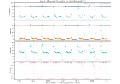
Flying Laptop: an empirical reference and its unexplained gap
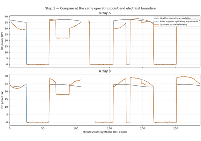
Expected versus actual power with known operating states
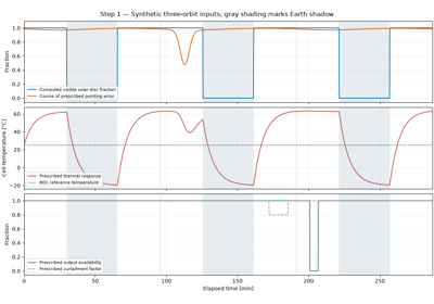
A spacecraft PV loss budget from orbit geometry to converter output
Real on-orbit data#
These examples retrieve and analyze public spacecraft telemetry rather than synthetic data.
Connector workflows#
Every walkthrough calls the public orbitalpv API and includes measured
coverage, source attribution, units and step-by-step figures. First runs
retrieve public files or API responses; later runs reuse local snapshots.
Source |
What is measured |
Example scope |
|---|---|---|
Flying Laptop |
Solar-array voltage and current; calculated V×I |
A month, 75,097 packet times and four arrays |
OPS-SAT-AD |
Photodiode/magnetometer signals and expert annotations |
303,493 values in 2,123 source segments |
TSIS-1 / SORCE TIM |
Total solar irradiance and uncertainty |
Annual history and instrument overlap, with missing bins preserved |
TSIS-1 SIM |
Wavelength-resolved solar irradiance and quality flags |
Three daily spectra, 2,104 wavelengths each |
NOAA GOES |
Integral proton/electron particle flux |
Seven-day measured environment snapshot |
BIRDS |
Panel voltage, current and temperature |
Four spacecraft and 48 flight campaigns |
Install pip install -U "orbital-pv[excel,examples]>=0.5.0". Flying Laptop
downloads approximately 30 MB and OPS-SAT approximately 19 MB once. Irradiance
and GOES examples request bounded subsets. The examples state when power is
computed from measured V/I or when a modeled PV response uses measured input.
For a held-out empirical reference comparison using the Flying Laptop measurements, see Flying Laptop reference gap. It reports signed power gaps, sampling coverage and observed-time energy while leaving physical causes unexplained when the required evidence is unavailable.
BIRDS campaign details#
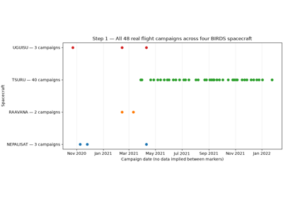
The BIRDS workflow uses measured solar-panel voltage, current and temperature from four 1U CubeSats: RAAVANA, UGUISU, NEPALISAT and TSURU. The source workbooks contain 48 flight campaigns, 31,725 measurement times and 158,625 panel observations. Each measurement time is counted within its spacecraft and campaign and contains five panel observations.
The walkthrough retains its original RAAVANA example address and includes:
an overview of all four spacecraft and their measurement coverage;
full-resolution plots of RAAVANA’s two approximately 90-minute campaigns, containing 1,079 and 1,080 measurements at five-second intervals;
five-minute power envelopes within each recorded campaign;
TSURU’s longer history of 40 flight campaigns.
TSURU’s two undated test sheets, Test1 w batt and Test2 wo batt, are
excluded. Its yearless March–December sheets use an explicitly inferred
campaign_year=2021, followed by the sheets explicitly dated January 2022.
This inference is consistent with TSURU’s 14 March 2021 deployment. The
normalized timestamps are campaign-date anchors plus recorded elapsed
seconds; the actual UTC session start is unknown. The example does not
interpolate measurements across campaign gaps or claim precise UTC timing.
The dataset is published by Jara and Lepcha (2022), DOI 10.17632/8kp25ycf63.1, under CC BY 4.0. Counts refer to the official source workbooks; the associated article describes the instrumentation and collection method.
Install the workbook reader and plotting dependencies with
pip install -U "orbital-pv[excel,examples]>=0.4.2". The first run downloads the
upstream workbooks and requires network access; subsequent runs reuse the
downloaded files. The public opv.fetch_birds_eps and
opv.load_birds_eps_workbook helpers both accept campaign_year=2021
for the TSURU yearless campaign names.
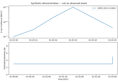
Solar activity: sunlight, X-rays and geomagnetic context
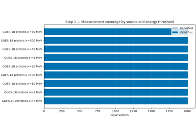
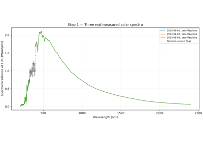
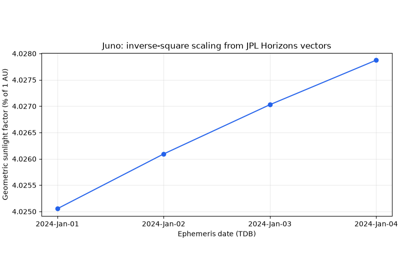
Free spacecraft research APIs: evidence, archives and geometry
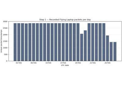
Flying Laptop: a month of measured solar-array generation
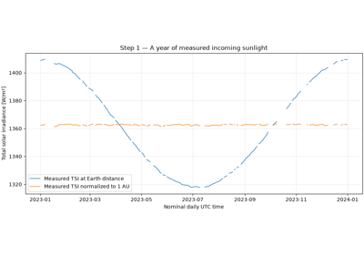
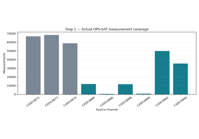
OPS-SAT photodiodes: real signals and expert annotations
Research physics and power systems#
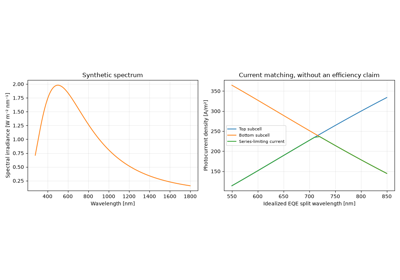
Explore transient thermal balance, radiation response, spectral current matching,
array circuits and battery-aware compute scheduling through the public
orbitalpv.physics API. These are reproducible screening scenarios with
declared assumptions. Synthetic spectra, circuit faults and mission profiles
are labeled explicitly; they are not flight measurements or exact reproductions
of the motivating research papers.
See Research physics: from photons to useful spacecraft power for equations, input units, validation limits and executable analyses.
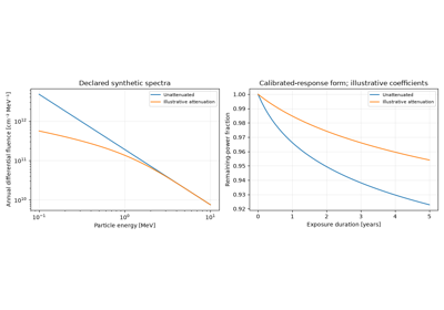
Integrate particle spectra before estimating remaining power
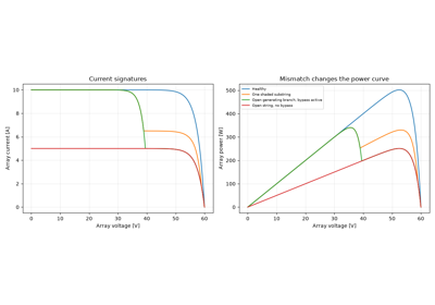
Distinguish mismatch, bypass and open-string I-V signatures
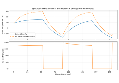
Follow panel temperature through sunlight and eclipse
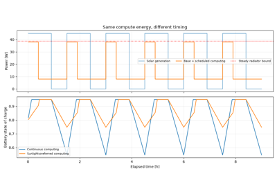
Schedule computing around sunlight and battery limits
Space PV business decisions#
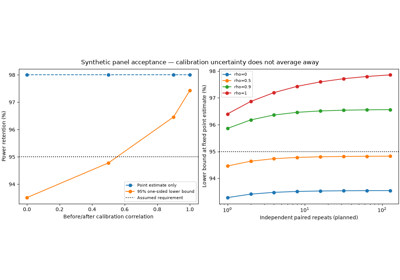
News-backed procurement and mission trade studies. Supplier claims motivate scenarios; modeled outputs and assumed economics are not flight qualification.
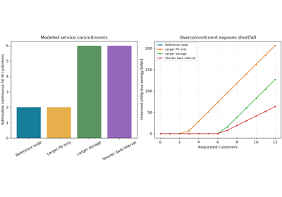
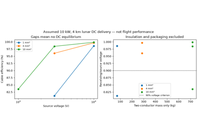
How much customer power can a lunar utility commit?
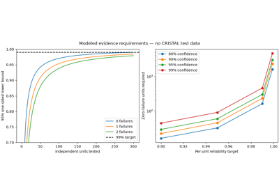
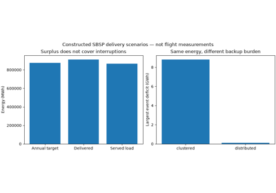
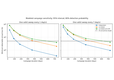
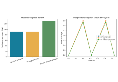
Does more solar power unlock continuous payload capacity?
Solar-powered AI clusters: links, formation, radiation and cost
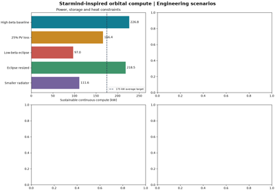
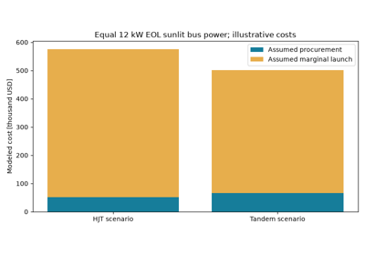
SpaceX Starmind: from HJT solar cells to usable orbital compute
Space cell technologies#
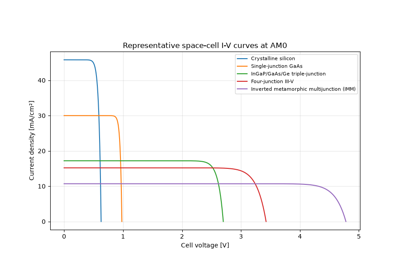
These examples compare representative space photovoltaic cell technologies through the public orbitalpv API.
The built-in templates cover five important technology families:
crystalline silicon;
single-junction GaAs;
InGaP/GaAs/Ge triple-junction;
four-junction III-V;
inverted metamorphic multijunction (IMM).
The models are intended for system studies, education and early design. They are not qualification models for a specific manufacturer part.
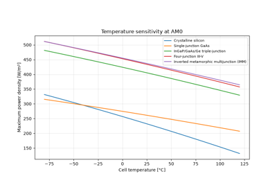
Temperature and radiation sensitivity of space cells