Note
Go to the end to download the full example code.
OPS-SAT photodiodes: real signals and expert annotations#
This example reads the original telemetry from the OPSSAT-AD v2 release,
using the public orbitalpv API. It contains 303,493 measurements in 2,123
segments from nine channels: three magnetometers and six photodiodes.
The photodiode channels add measured illumination/attitude-related context to
OrbitalPV; they are not solar-panel electrical power measurements.
Source and interpretation#
Ruszczak et al. (2025), The OPS-SAT benchmark for detecting anomalies in satellite telemetry, https://doi.org/10.1038/s41597-025-05035-3.
Original measurement CSV, version v2 (CC BY 4.0): https://doi.org/10.5281/zenodo.15108715.
We use
segments.csv, not the separate derived-feature tabledataset.csv. No synthetic measurements are added.
The CSV supplies UTC timestamps and values but no engineering-unit field.
Values therefore stay in their published scale, labeled source units.
Photodiode channel names ending in THETA are preserved; we do not infer
irradiance, electrical current, power, or a calibrated angle unit from them.
The source is a curated selection of nominal and anomalous segments, not a continuous mission log. We preserve its segment boundaries, missing periods, and original training/test split. The expert labels describe this benchmark; the example does not make a new anomaly diagnosis or estimate fleet failure rates.
from __future__ import annotations

from pathlib import Path
from tempfile import gettempdir

import matplotlib.pyplot as plt
import numpy as np

import orbitalpv as opv
The connector downloads the pinned 19 MB CSV once, checks its SHA-256 hash,
and keeps a provenance sidecar. A subsequent run reuses the verified cache.
It returns all published measurements; filtering can also be requested with
channels=["CADC0892"] and split="test".
cache = Path(gettempdir()) / "orbitalpv-real-data"
with opv.OpsSatADConnector() as connector:
    telemetry = connector.download_frame(cache / "opssat_segments_v2.csv")

segments = telemetry.drop_duplicates("segment")
print(f"Measurements: {len(telemetry):,}")
print(f"Source segments: {len(segments):,}")
print(f"Channels: {telemetry['channel'].nunique()}")
print(f"UTC coverage: {telemetry['timestamp'].min()} to {telemetry['timestamp'].max()}")
print(f"Source: {telemetry.attrs['source_doi']} ({telemetry.attrs['license']})")
print(f"Complete-release checksum verified: {telemetry.attrs['matches_complete_release']}")

counts = telemetry.groupby(["channel", "sensor_type"], sort=True).size()
fig, ax = plt.subplots(figsize=(10, 4.5))
ax.bar(
    counts.index.get_level_values("channel"),
    counts.to_numpy(),
    color=["#167d8d" if kind == "photodiode" else "#7a8795" for _, kind in counts.index],
)
ax.set(
    title="Step 1 — Actual OPS-SAT measurement coverage",
    xlabel="Source channel",
    ylabel="Measurements",
)
ax.tick_params(axis="x", rotation=35)
ax.grid(axis="y", alpha=0.25)
fig.tight_layout()
plt.show()
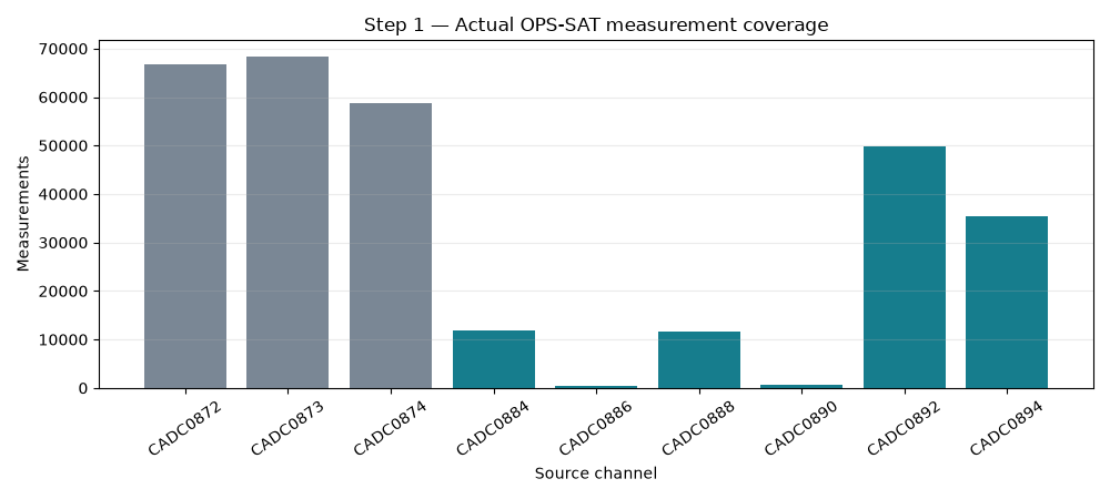
Measurements: 303,493
Source segments: 2,123
Channels: 9
UTC coverage: 2022-01-04 20:00:50+00:00 to 2022-06-02 15:10:42+00:00
Source: 10.5281/zenodo.15108715 (CC-BY-4.0)
Complete-release checksum verified: True
These plots use every available photodiode measurement on its original UTC timestamp. Points leave unobserved periods blank; no line or interpolation bridges separate telemetry segments. Each channel retains its source value scale, so the y-axis is deliberately not labeled in watts or amperes.
photodiodes = telemetry[telemetry["sensor_type"].eq("photodiode")].copy()
print(f"Photodiode measurements: {len(photodiodes):,}")
fig, axes = plt.subplots(3, 2, figsize=(12, 9), sharex=True, sharey=True)
for ax, (channel, samples) in zip(
    axes.flat, photodiodes.groupby("channel", sort=True), strict=True
):
    ax.plot(samples["timestamp"], samples["value"], ".", markersize=1.5, alpha=0.5, color="#167d8d")
    ax.set_title(f"{channel} · {samples['channel_name'].iloc[0]}", fontsize=10)
    ax.set_ylabel("Source value [unit unspecified]")
    ax.grid(alpha=0.2)
for ax in axes[-1]:
    ax.set_xlabel("Source UTC time")
    ax.tick_params(axis="x", rotation=25)
fig.suptitle("Step 2 — All published photodiode samples; gaps remain visible")
fig.tight_layout()
plt.show()
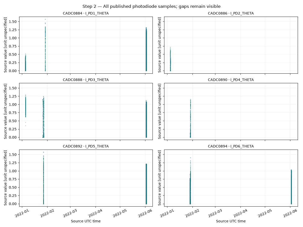
Photodiode measurements: 109,666
We select the longest nominal and longest anomalous segment of CADC0892, making the choice reproducible. Each panel shows a separate segment against its actual elapsed seconds; a scatter plot keeps missing samples visible.
Use the numeric ``anomaly`` column for the expert label. The source v2
text column label says "anomaly" for nominal rows too. OrbitalPV
preserves that field for provenance but does not use it for classification.
channel_samples = photodiodes[photodiodes["channel"].eq("CADC0892")]
sizes = channel_samples.groupby(["anomaly", "segment"]).size()
fig, axes = plt.subplots(1, 2, figsize=(12, 4.3), sharey=True)
for annotation, ax in enumerate(axes):
    segment_id = int(sizes.loc[annotation].idxmax())
    samples = channel_samples[channel_samples["segment"].eq(segment_id)].sort_values("timestamp")
    elapsed = (samples["timestamp"] - samples["timestamp"].iloc[0]).dt.total_seconds()
    color = "#ba4a40" if annotation else "#167d8d"
    label = "Anomalous" if annotation else "Nominal"
    ax.plot(elapsed, samples["value"], ".", markersize=3, color=color)
    ax.set(
        title=f"{label} source annotation · segment {segment_id}",
        xlabel="Elapsed seconds within this segment",
        ylabel="I_PD5_THETA [source unit unspecified]",
    )
    ax.grid(alpha=0.2)
    print(
        f"{label}: segment {segment_id}, {len(samples)} measurements, starts {samples['timestamp'].iloc[0]}"
    )
fig.suptitle("Step 3 — Published expert labels, not a new model diagnosis")
fig.tight_layout()
plt.show()
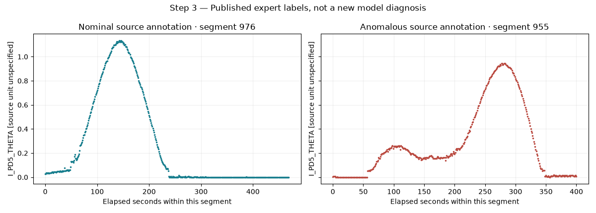
Nominal: segment 976, 470 measurements, starts 2022-06-02 09:44:15+00:00
Anomalous: segment 955, 401 measurements, starts 2022-06-02 08:10:34+00:00
Count segments, not individual samples, when summarizing the expert annotations. Segment lengths vary. The curated anomaly prevalence is not a mission-wide anomaly or failure rate. The original train/test assignment is kept intact and must not be confused with a chronological holdout.
photodiode_segments = photodiodes.drop_duplicates("segment")
by_channel = (
    photodiode_segments.groupby(["channel", "anomaly"])
    .size()
    .unstack(fill_value=0)
    .reindex(columns=[0, 1], fill_value=0)
)
by_split = (
    segments.assign(split=np.where(segments["train"].eq(1), "Training", "Test"))
    .groupby(["split", "anomaly"])
    .size()
    .unstack(fill_value=0)
    .reindex(index=["Training", "Test"], columns=[0, 1], fill_value=0)
)
fig, axes = plt.subplots(1, 2, figsize=(12, 4.5))
for ax, summary, title in zip(
    axes,
    [by_channel, by_split],
    ["Photodiode source segments", "All channels: published benchmark split"],
    strict=True,
):
    summary.rename(columns={0: "Nominal", 1: "Anomalous"}).plot.bar(
        ax=ax,
        stacked=True,
        color=["#167d8d", "#ba4a40"],
        rot=30,
    )
    ax.set(title=title, xlabel="", ylabel="Source segments")
    ax.grid(axis="y", alpha=0.25)
fig.suptitle("Step 4 — Curated labels and source split remain unchanged")
fig.tight_layout()
plt.show()

print("\nPublished segment split (numeric anomaly annotation):")
print(by_split.rename(columns={0: "nominal", 1: "anomalous"}).to_string())

# These measured signals can support studies of telemetry quality, sensor
# behavior, and illumination-related operating conditions. Calculating PV
# output would additionally require validated sensor calibration, geometry,
# panel electrical measurements, and a suitable PV model.
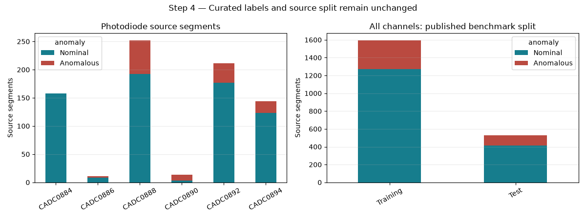
Published segment split (numeric anomaly annotation):
anomaly   nominal  anomalous
split
Training     1273        321
Test          416        113
Total running time of the script: (0 minutes 4.422 seconds)