Note
Go to the end to download the full example code.
Measured solar irradiance from TSIS-1 and SORCE#
Retrieve real, calibrated total solar irradiance (TSI) measurements from LASP LISIRD and use them as an input to an illustrative PV calculation. TSIS-1/TIM measures sunlight from the International Space Station; SORCE/TIM provides an independent spacecraft record. These are measured incoming solar irradiance, in W/m². The final DC-power curve is explicitly a model.
This example requests a complete year of daily TSIS-1 data (2023), followed by a 2019 overlap with SORCE. Fixed historical intervals and cached raw JSON make the retrieval reproducible. The source can revise historical calibration, so each cache retains its request, retrieval time, original metadata and SHA-256 checksum. No measurements are interpolated across missing days.
Sources#
TSIS-1/TIM daily data and acknowledgments: https://lasp.colorado.edu/lisird/data/tsis_tsi_24hr/
SORCE/TIM daily data and acknowledgments: https://lasp.colorado.edu/lisird/data/sorce_tsi_24hr_l3/
Product descriptions and release notes: https://lasp.colorado.edu/tsis/data/ and https://lasp.colorado.edu/sorce/data/.
Kopp, G. (2025), TSIS TIM Level 3 Total Solar Irradiance 24-hour Means, version 05, NASA GES DISC. Retain LASP and instrument-team attribution.
The returned timestamp is the nominal center of a daily averaging
interval, not an instantaneous detector reading. The source’s weighted
average measurement time is preserved separately. Measurements normalized to
1 AU and measurements corrected to the actual Earth–Sun distance are kept
separate; the latter already include the distance effect.
from pathlib import Path
from tempfile import gettempdir

import matplotlib.pyplot as plt
import numpy as np
import pandas as pd

import orbitalpv as opv
The connector reads the time units and fill values from the source response. TSI=0 is the provider’s missing-data value, not a spacecraft eclipse. Missing irradiances become NaN. Provisional flags and source uncertainties remain available for inspection; the dates here use a historical release.
cache = Path(gettempdir()) / "orbitalpv-lisird"
with opv.LisirdConnector() as connector:
    measured = connector.total_solar_irradiance(
        "tsis_tsi_24hr",
        time_min="2023-01-01",
        time_max="2024-01-01",
        cache_path=cache / "tsis_tsi_24hr-2023-01-01.json",
    )

print(
    f"Daily bins: {len(measured):,}; valid measured bins: {int(measured['valid_measurement'].sum()):,}"
)
print(f"Nominal UTC time range: {measured['timestamp'].min()} to {measured['timestamp'].max()}")
print(f"Raw-response SHA256: {measured.attrs['provenance']['sha256']}")
print(
    "Source provisional flags:", measured["provisional_flag"].value_counts(dropna=False).to_dict()
)

fig, ax = plt.subplots(figsize=(10, 4.6), layout="constrained")
ax.plot(
    measured["timestamp"],
    measured["tsi_earth_w_m2"],
    label="Measured TSI at Earth distance",
    linewidth=1.1,
)
ax.plot(
    measured["timestamp"],
    measured["tsi_1au_w_m2"],
    label="Measured TSI normalized to 1 AU",
    linewidth=1.1,
)
ax.set(
    xlabel="Nominal daily UTC time",
    ylabel="Total solar irradiance [W/m²]",
    title="Step 1 — A year of measured incoming sunlight",
)
ax.grid(alpha=0.25)
ax.legend()
plt.show()
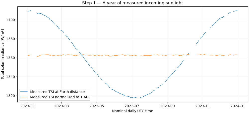
Daily bins: 365; valid measured bins: 292
Nominal UTC time range: 2023-01-01 12:00:00+00:00 to 2023-12-31 12:00:00+00:00
Raw-response SHA256: 79f7635862186d70eec63b8934523fbdb57683be4f37c20d30fd6313bc8cee2b
Source provisional flags: {0: 365}
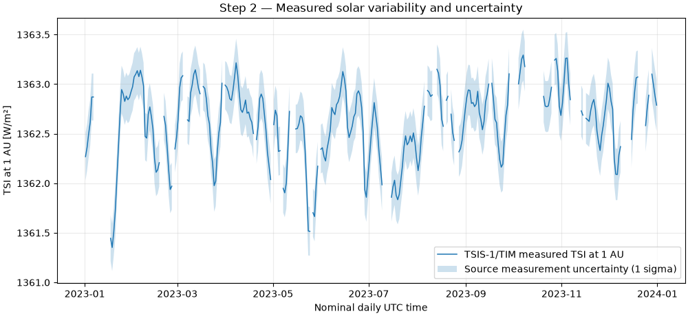
Removing the known solar-distance effect exposes much smaller intrinsic changes in the Sun. The shaded interval is the source’s reported 1-sigma measurement uncertainty. It is not a confidence interval for a fitted model.
fig, ax = plt.subplots(figsize=(10, 4.6), layout="constrained")
time = measured["timestamp"]
irradiance = measured["tsi_1au_w_m2"].to_numpy(dtype=float)
uncertainty = measured["uncertainty_1au_w_m2"].to_numpy(dtype=float)
ax.plot(time, irradiance, linewidth=1.1, label="TSIS-1/TIM measured TSI at 1 AU")
ax.fill_between(
    time,
    irradiance - uncertainty,
    irradiance + uncertainty,
    alpha=0.22,
    label="Source measurement uncertainty (1 sigma)",
)
ax.set(
    xlabel="Nominal daily UTC time",
    ylabel="TSI at 1 AU [W/m²]",
    title="Step 2 — Measured solar variability and uncertainty",
)
ax.grid(alpha=0.25)
ax.legend()
plt.show()
The overlap checks two instruments observing the same solar input. Their absolute scales and uncertainties differ, so do not splice them into one supposedly homogeneous series without a cross-calibration method. Align nominal daily bins exactly; no nearest-date matching or gap filling is used.
with opv.LisirdConnector() as connector:
    tsis_overlap = connector.total_solar_irradiance(
        "tsis_tsi_24hr",
        time_min="2019-01-01",
        time_max="2020-01-01",
        cache_path=cache / "tsis_tsi_24hr-2019-01-01.json",
    )
    sorce_overlap = connector.total_solar_irradiance(
        "sorce_tsi_24hr_l3",
        time_min="2019-01-01",
        time_max="2020-01-01",
        cache_path=cache / "sorce_tsi_24hr_l3-2019-01-01.json",
    )
comparison = pd.merge(
    tsis_overlap[["timestamp", "tsi_1au_w_m2"]],
    sorce_overlap[["timestamp", "tsi_1au_w_m2"]],
    on="timestamp",
    how="outer",
    suffixes=("_tsis", "_sorce"),
    validate="one_to_one",
).sort_values("timestamp")
comparison["difference_w_m2"] = comparison["tsi_1au_w_m2_tsis"] - comparison["tsi_1au_w_m2_sorce"]
print(f"Overlapping valid daily pairs: {int(comparison['difference_w_m2'].notna().sum()):,}")
print(f"Mean TSIS minus SORCE: {comparison['difference_w_m2'].mean():.4f} W/m²")

fig, axes = plt.subplots(2, 1, figsize=(10, 7), sharex=True, layout="constrained")
axes[0].plot(
    comparison["timestamp"], comparison["tsi_1au_w_m2_tsis"], linewidth=1, label="TSIS-1/TIM"
)
axes[0].plot(
    comparison["timestamp"], comparison["tsi_1au_w_m2_sorce"], linewidth=1, label="SORCE/TIM"
)
axes[0].set(ylabel="Measured TSI at 1 AU [W/m²]", title="Step 3 — Independent instrument overlap")
axes[0].legend()
axes[1].plot(comparison["timestamp"], comparison["difference_w_m2"], linewidth=1, color="#6A4C93")
axes[1].axhline(0, color="black", linewidth=0.8)
axes[1].set(xlabel="Nominal daily UTC time", ylabel="TSIS - SORCE [W/m²]")
for ax in axes:
    ax.grid(alpha=0.25)
plt.show()
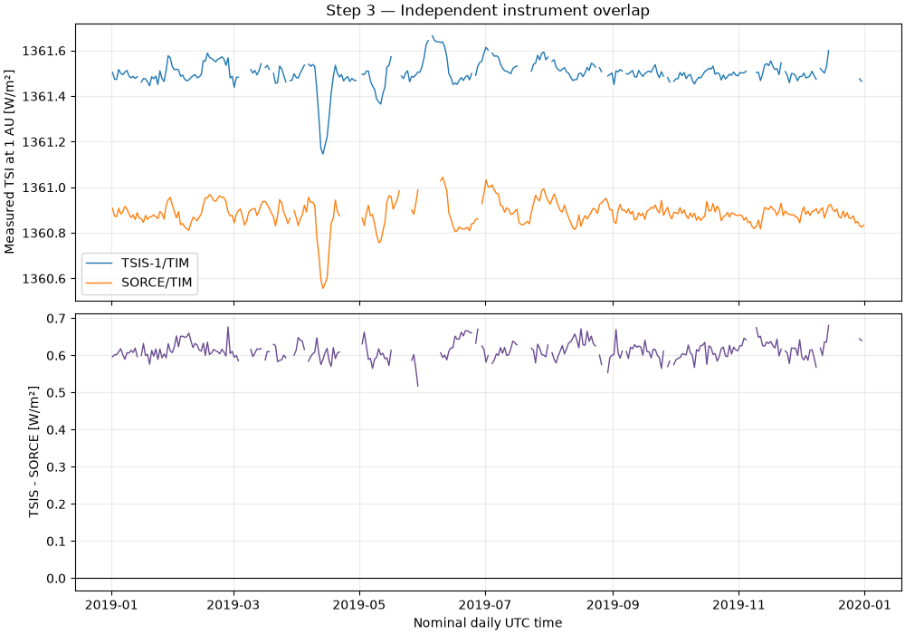
Overlapping valid daily pairs: 290
Mean TSIS minus SORCE: 0.6134 W/m²
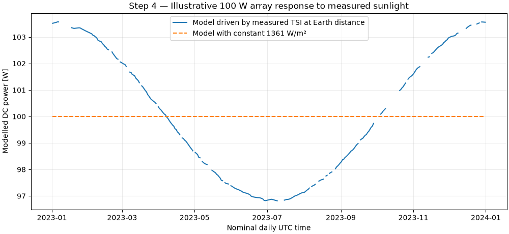
A 100 W reference array, defined at 1361 W/m² and 25°C, is held normal to the Sun at constant cell temperature with no eclipse or optical losses. These are stated model assumptions, not TSIS hardware specifications. The result is modelled DC power, not measured panel power or mission energy production. Use the Earth-distance irradiance directly: applying inverse-square solar distance scaling again would double-count an effect already in the data.
reference = opv.PvwattsReference(
    pdc0_w=100.0,
    gamma_pdc_per_c=-0.003,
    reference_irradiance_w_m2=1361.0,
    reference_temperature_c=25.0,
)
modelled_dc_w = opv.pvwatts_dc_space(
    measured["tsi_earth_w_m2"].to_numpy(dtype=float), 25.0, reference
)
constant_dc_w = opv.pvwatts_dc_space(np.full(len(measured), 1361.0), 25.0, reference)

fig, ax = plt.subplots(figsize=(10, 4.6), layout="constrained")
ax.plot(
    measured["timestamp"], modelled_dc_w, label="Model driven by measured TSI at Earth distance"
)
ax.plot(measured["timestamp"], constant_dc_w, linestyle="--", label="Model with constant 1361 W/m²")
ax.set(
    xlabel="Nominal daily UTC time",
    ylabel="Modelled DC power [W]",
    title="Step 4 — Illustrative 100 W array response to measured sunlight",
)
ax.grid(alpha=0.25)
ax.legend()
plt.show()
Total running time of the script: (0 minutes 8.522 seconds)