Note
Go to the end to download the full example code.
Real BIRDS CubeSat solar-panel telemetry#
Analyze all four BIRDS spacecraft through the public orbitalpv API,
with full-resolution RAAVANA traces and a longer TSURU campaign history.
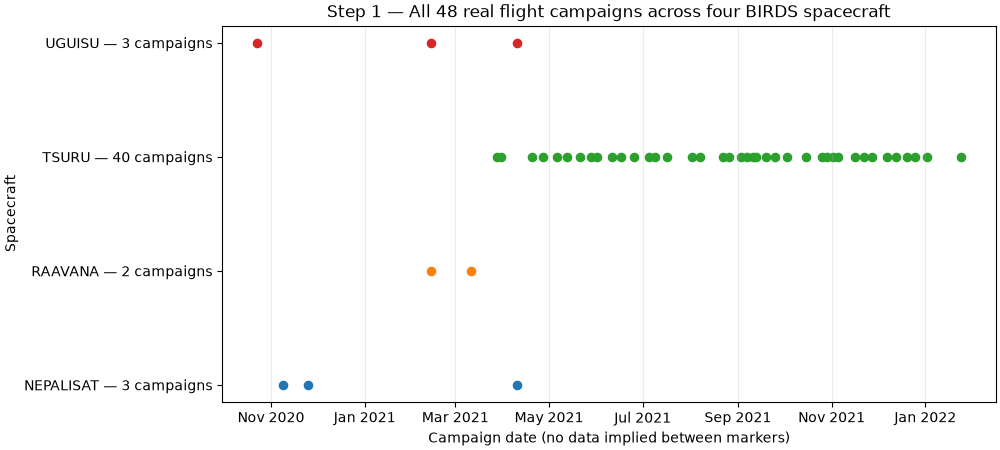
The published workbooks contain 48 flight campaigns, 31,725 measurement
times and 158,625 panel observations across five faces per spacecraft.
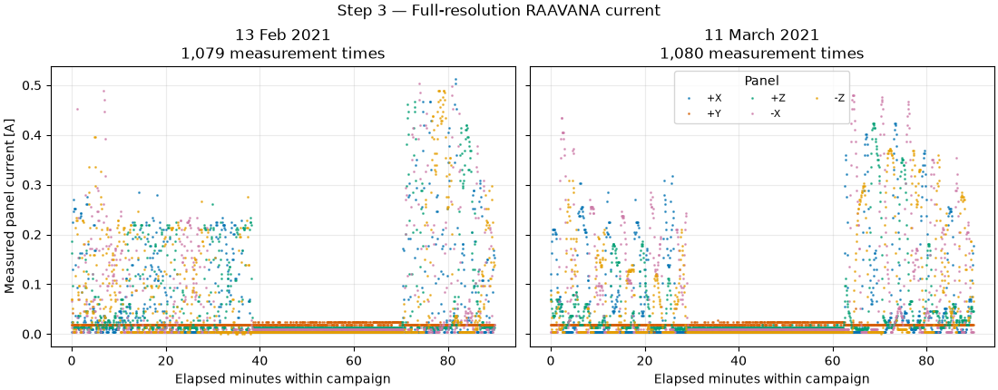
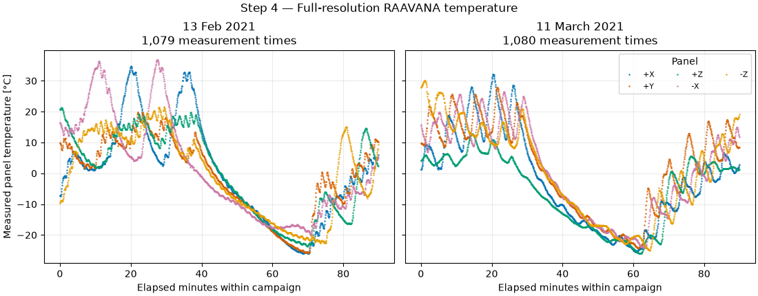
RAAVANA has only two campaigns, but they contain 2,159 measurement times, mostly hidden when plotted on a month-wide date axis. Here we show every native sample against elapsed minutes, add within-campaign summaries, and use TSURU’s 40 flight campaigns for the longer comparison. No samples are interpolated or invented between campaigns.
Install pip install -U "orbital-pv[excel,examples]>=0.4.2". The first run downloads
the original workbooks; later runs reuse the local copies. Delete a cached
workbook to fetch it again. Printed checksums identify the input files.
Source and time interpretation#
Jara et al. (2022), On-orbit Electrical Power System Dataset of 1U CubeSat constellation for Machine Learning Models.
Dataset: https://doi.org/10.17632/8kp25ycf63.1 (CC BY 4.0).
Workbooks: BIRDSOpenSource/EPS_dataset.
Acquisition details: https://pmc.ncbi.nlm.nih.gov/articles/PMC9679683/.
The workbooks give campaign dates and elapsed seconds, not a known UTC
clock start. The connector’s timestamp is a calendar-date anchor plus
the supplied elapsed seconds. We use dates for campaign summaries and elapsed
minutes for detailed traces; these reconstructed timestamps must not be
joined directly to orbit/attitude data as precise acquisition times.
TSURU’s March–December sheet names omit a year. We explicitly assign 2021,
an inference consistent with its March 2021 deployment and the following
January 2022 sheets. The two sheets named Test1 w batt and Test2 wo batt
are excluded from flight analysis. Dates that already include a year retain
it. Campaigns are sorted by date, since workbook order is not chronological.
All health comparisons remain exploratory: attitude, illumination, thermal state and operating conditions are not normalized. More measurements do not, by themselves, establish a degradation rate or a fault diagnosis.
from __future__ import annotations

from hashlib import sha256
from pathlib import Path
from tempfile import gettempdir

import matplotlib.dates as mdates
import matplotlib.pyplot as plt
import numpy as np
import pandas as pd

import orbitalpv as opv
Each measurement time contributes five panel rows. Count the two quantities separately, retaining spacecraft and campaign identity throughout. The explicit TSURU year applies only to sheet dates that omit their year.
cache = Path(gettempdir()) / "orbitalpv-real-data"
cache.mkdir(parents=True, exist_ok=True)
satellite_years = {"RAAVANA": None, "UGUISU": None, "NEPALISAT": None, "TSURU": 2021}
frames = []
for satellite, campaign_year in satellite_years.items():
    workbook = cache / f"{satellite}.xlsx"
    if workbook.exists():
        frame = opv.load_birds_eps_workbook(workbook, campaign_year=campaign_year)
    else:
        frame = opv.fetch_birds_eps(satellite, workbook, campaign_year=campaign_year)
    frame["satellite"] = satellite
    frames.append(frame)
    print(f"{satellite}.xlsx SHA256={sha256(workbook.read_bytes()).hexdigest()}")

telemetry = pd.concat(frames, ignore_index=True)
telemetry = telemetry.sort_values(
    ["satellite", "campaign_date", "panel_id", "elapsed_seconds"]
).reset_index(drop=True)
powered = opv.add_power(telemetry)
powered = powered[np.isfinite(powered["power_w"])].copy()

measurement_times = telemetry.drop_duplicates(["satellite", "source_sheet", "elapsed_seconds"])
campaigns = (
    measurement_times.groupby(["satellite", "source_sheet"], as_index=False)
    .agg(
        campaign_date=("campaign_date", "first"),
        measurement_times=("elapsed_seconds", "size"),
        first_second=("elapsed_seconds", "min"),
        last_second=("elapsed_seconds", "max"),
    )
    .sort_values(["satellite", "campaign_date"])
)
campaigns["duration_minutes"] = (campaigns["last_second"] - campaigns["first_second"]) / 60
coverage = campaigns.groupby("satellite").agg(
    flight_campaigns=("source_sheet", "size"),
    measurement_times=("measurement_times", "sum"),
    first_campaign=("campaign_date", "min"),
    last_campaign=("campaign_date", "max"),
)
coverage["panel_observations"] = telemetry.groupby("satellite").size()
print(coverage.to_string())
print(
    f"Total: {len(campaigns):,} flight campaigns; "
    f"{len(measurement_times):,} measurement times; {len(telemetry):,} panel observations"
)
print("Campaign dates are calendar anchors; absolute UTC acquisition times are unknown.")

fig, ax = plt.subplots(figsize=(10, 4.5), layout="constrained")
for row, (satellite, group) in enumerate(campaigns.groupby("satellite", sort=True)):
    ax.scatter(group["campaign_date"], np.full(len(group), row), s=35, label=satellite)
ax.set(
    xlabel="Campaign date (no data implied between markers)",
    ylabel="Spacecraft",
    yticks=range(len(coverage)),
    yticklabels=[
        f"{name} — {count} campaigns" for name, count in coverage["flight_campaigns"].items()
    ],
    title="Step 1 — All 48 real flight campaigns across four BIRDS spacecraft",
)
ax.xaxis.set_major_locator(mdates.MonthLocator(interval=2))
ax.xaxis.set_major_formatter(mdates.DateFormatter("%b %Y"))
ax.grid(True, axis="x", alpha=0.25)
plt.show()
RAAVANA.xlsx SHA256=439edd8a824ff4829d7d2fddd44eb7559fc553cde8726c4eb2860d9b11543035
UGUISU.xlsx SHA256=4eac4d50e584ac96ba94936b6cd6fe6140b3ab862153b87408bd6911ca88c140
NEPALISAT.xlsx SHA256=89ff16ba152712073537ab0bd6a8d653387bfdaf6f38aa19af9a30e2f2699d59
TSURU.xlsx SHA256=a92442de22185ebeb7964e82ae77a45a9cd59e23606833e8caaf5b81818e353a
           flight_campaigns  measurement_times            first_campaign             last_campaign  panel_observations
satellite
NEPALISAT                 3               3040 2020-11-09 00:00:00+00:00 2021-04-10 00:00:00+00:00               15200
RAAVANA                   2               2159 2021-02-13 00:00:00+00:00 2021-03-11 00:00:00+00:00               10795
TSURU                    40              23266 2021-03-28 00:00:00+00:00 2022-01-24 00:00:00+00:00              116330
UGUISU                    3               3260 2020-10-23 00:00:00+00:00 2021-04-10 00:00:00+00:00               16300
Total: 48 flight campaigns; 31,725 measurement times; 158,625 panel observations
Campaign dates are calendar anchors; absolute UTC acquisition times are unknown.
Each subplot contains one complete recording at the native five-second cadence. Separate axes make the thousands of samples visible without drawing a line across the 26-day gap. Colors and panel labels remain consistent in every subsequent figure.
panel_colors = dict(
    zip(
        sorted(telemetry["panel_id"].unique()),
        ["#0072B2", "#D55E00", "#009E73", "#CC79A7", "#E69F00"],
        strict=True,
    )
)
raavana = powered[powered["satellite"] == "RAAVANA"].copy()
raavana_campaigns = campaigns[campaigns["satellite"] == "RAAVANA"]
print("\nRAAVANA native recording coverage")
print(raavana_campaigns.to_string(index=False))


def plot_raavana_quantity(column: str, ylabel: str, title: str) -> None:
    """Show every sample separately within each RAAVANA flight campaign."""
    fig, axes = plt.subplots(
        1, len(raavana_campaigns), figsize=(11, 4.3), sharey=True, layout="constrained"
    )
    for ax, campaign in zip(np.atleast_1d(axes), raavana_campaigns.itertuples(), strict=True):
        session = raavana[raavana["source_sheet"] == campaign.source_sheet]
        for panel_id, panel in session.groupby("panel_id", sort=True):
            ax.plot(
                panel["elapsed_seconds"] / 60,
                panel[column],
                ".",
                ms=2,
                alpha=0.65,
                color=panel_colors[panel_id],
                label=panel_id,
            )
        ax.set(
            title=f"{campaign.source_sheet}\n{campaign.measurement_times:,} measurement times",
            xlabel="Elapsed minutes within campaign",
        )
        ax.grid(True, alpha=0.25)
    axes[0].set_ylabel(ylabel)
    axes[-1].legend(title="Panel", fontsize=8, ncols=3)
    fig.suptitle(title)
    plt.show()


plot_raavana_quantity(
    "voltage_v", "Measured panel voltage [V]", "Step 2 — Full-resolution RAAVANA voltage"
)
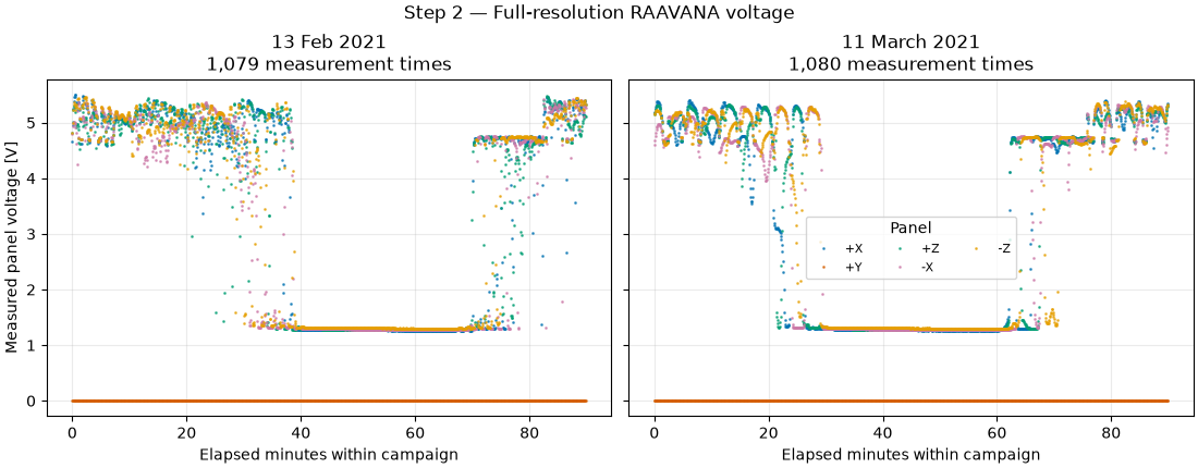
RAAVANA native recording coverage
satellite  source_sheet             campaign_date  measurement_times  first_second  last_second  duration_minutes
  RAAVANA   13 Feb 2021 2021-02-13 00:00:00+00:00               1079           0.0       5390.0         89.833333
  RAAVANA 11 March 2021 2021-03-11 00:00:00+00:00               1080           0.0       5395.0         89.916667
These are calibrated currents from the workbook, converted from mA to A.
plot_raavana_quantity(
    "current_a", "Measured panel current [A]", "Step 3 — Full-resolution RAAVANA current"
)
Temperature helps put changes in electrical output in context; it is not a correction for spacecraft attitude or solar incidence.
plot_raavana_quantity(
    "temperature_c",
    "Measured panel temperature [°C]",
    "Step 4 — Full-resolution RAAVANA temperature",
)
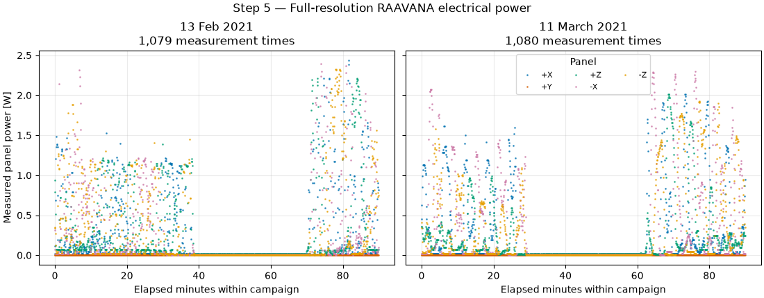
opv.add_power calculates P = V x I. We retain the complete measured signal
within each campaign, including low-power intervals. No orbital eclipse or
fault labels are inferred from those intervals alone.
plot_raavana_quantity(
    "power_w", "Measured panel power [W]", "Step 5 — Full-resolution RAAVANA electrical power"
)
Five-minute, non-overlapping windows expose changes within each RAAVANA recording. A window needs at least 30 valid panel samples (half the expected 60 samples at five-second cadence); the final window is retained if it meets that requirement. Windows are always grouped by spacecraft, campaign and panel, so none can span the gap between recordings. These local P95 values describe short-term operating behavior, not an independent health verdict.
window_seconds = 300
minimum_window_samples = 30
raavana["window_start_s"] = np.floor(raavana["elapsed_seconds"] / window_seconds) * window_seconds
window_p95 = raavana.groupby(
    ["satellite", "source_sheet", "panel_id", "window_start_s"], as_index=False
).agg(
    power_p95_w=("power_w", lambda values: float(values.quantile(0.95))),
    samples=("power_w", "size"),
)
window_p95 = window_p95[window_p95["samples"] >= minimum_window_samples]
window_count = len(window_p95.drop_duplicates(["satellite", "source_sheet", "window_start_s"]))
print(
    f"\nRAAVANA: {window_count} within-campaign time windows; {len(window_p95)} panel-window summaries"
)

fig, axes = plt.subplots(
    1, len(raavana_campaigns), figsize=(11, 4.3), sharey=True, layout="constrained"
)
for ax, campaign in zip(axes, raavana_campaigns.itertuples(), strict=True):
    session = window_p95[window_p95["source_sheet"] == campaign.source_sheet]
    for panel_id, panel in session.groupby("panel_id", sort=True):
        ax.scatter(
            panel["window_start_s"] / 60,
            panel["power_p95_w"],
            s=22,
            color=panel_colors[panel_id],
            label=panel_id,
        )
    ax.set(title=campaign.source_sheet, xlabel="Window start [elapsed minutes]")
    ax.grid(True, alpha=0.25)
axes[0].set_ylabel("Five-minute 95th-percentile power [W]")
axes[-1].legend(title="Panel", fontsize=8, ncols=3)
fig.suptitle(f"Step 6 — {window_count} real time windows, separated by campaign")
plt.show()
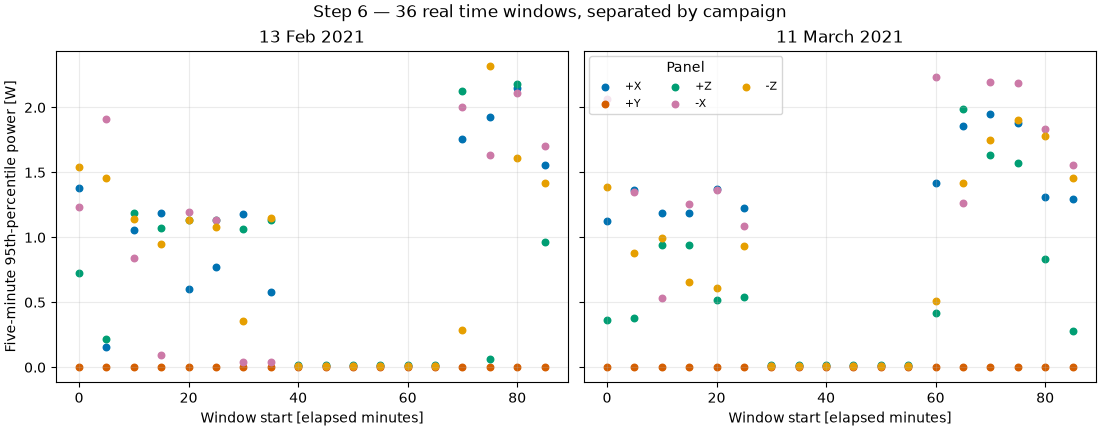
RAAVANA: 36 within-campaign time windows; 180 panel-window summaries
Compute campaign summaries using every valid measurement from all four spacecraft. TSURU supplies a longer March 2021–January 2022 comparison. Marker-only plots avoid suggesting continuous coverage between campaigns. The bars above show how many native measurement times support each point.
session_p95 = (
    powered.groupby(["satellite", "panel_id", "source_sheet", "campaign_date"], as_index=False)
    .agg(
        power_p95_w=("power_w", lambda values: float(values.quantile(0.95))),
        samples=("power_w", "size"),
    )
    .sort_values(["satellite", "panel_id", "campaign_date"])
)
tsuru_sessions = session_p95[session_p95["satellite"] == "TSURU"]
tsuru_campaigns = campaigns[campaigns["satellite"] == "TSURU"]

fig, axes = plt.subplots(
    2, 1, figsize=(10, 7), sharex=True, layout="constrained", gridspec_kw={"height_ratios": [1, 2]}
)
axes[0].bar(
    tsuru_campaigns["campaign_date"],
    tsuru_campaigns["measurement_times"],
    width=2.5,
    color="#586A83",
)
axes[0].set(ylabel="Measurement times", title="Step 7 — TSURU: 40 real flight campaigns")
for panel_id, panel in tsuru_sessions.groupby("panel_id", sort=True):
    axes[1].scatter(
        panel["campaign_date"],
        panel["power_p95_w"],
        s=24,
        color=panel_colors[panel_id],
        label=panel_id,
    )
axes[1].set(
    xlabel="Campaign date (2021 inferred for yearless sheets)",
    ylabel="Campaign 95th-percentile power [W]",
)
axes[1].xaxis.set_major_locator(mdates.MonthLocator(interval=2))
axes[1].xaxis.set_major_formatter(mdates.DateFormatter("%b %Y"))
axes[1].legend(title="Panel", fontsize=8, ncols=5)
for ax in axes:
    ax.grid(True, alpha=0.25)
plt.show()
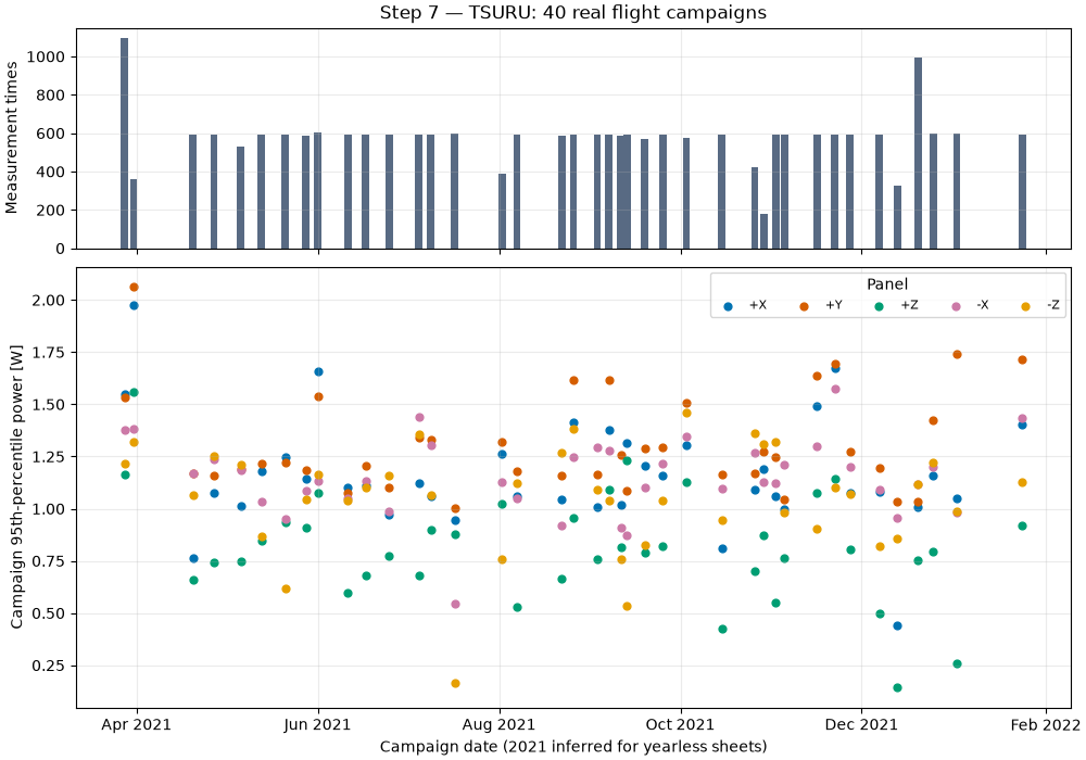
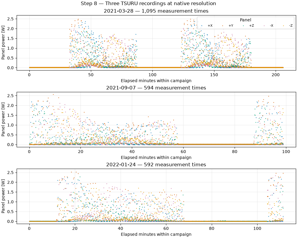
The campaign summaries above use all 23,266 TSURU measurement times. For detailed comparison, display every native sample from three representative recordings. Preserve the workbook’s actual elapsed values, including its fractional-second sampling intervals, instead of imposing a fixed cadence.
selected_tsuru = tsuru_campaigns.iloc[[0, len(tsuru_campaigns) // 2, -1]]
fig, axes = plt.subplots(3, 1, figsize=(10, 8), sharey=True, layout="constrained")
for ax, campaign in zip(axes, selected_tsuru.itertuples(), strict=True):
    session = powered[
        (powered["satellite"] == "TSURU") & (powered["source_sheet"] == campaign.source_sheet)
    ]
    for panel_id, panel in session.groupby("panel_id", sort=True):
        ax.plot(
            panel["elapsed_seconds"] / 60,
            panel["power_w"],
            ".",
            ms=2,
            alpha=0.65,
            color=panel_colors[panel_id],
            label=panel_id,
        )
    ax.set(
        title=f"{campaign.campaign_date:%Y-%m-%d} — {campaign.measurement_times:,} measurement times",
        xlabel="Elapsed minutes within campaign",
        ylabel="Panel power [W]",
    )
    ax.grid(True, alpha=0.25)
axes[0].legend(title="Panel", fontsize=8, ncols=5)
fig.suptitle("Step 8 — Three TSURU recordings at native resolution")
plt.show()
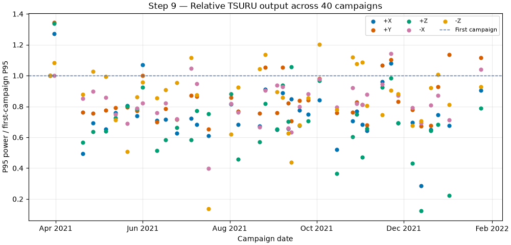
Normalize each face to its own first campaign P95. This extends the former two-point view to 40 campaign points per face. The reference is a measured operating state, not a proven healthy baseline. Changes in illumination and attitude can move this ratio; no degradation rate is fitted to it.
tsuru_relative = tsuru_sessions.copy()
reference = tsuru_relative.groupby("panel_id")["power_p95_w"].transform("first")
tsuru_relative["relative_envelope"] = tsuru_relative["power_p95_w"] / reference.where(reference > 0)

fig, ax = plt.subplots(figsize=(10, 4.8), layout="constrained")
for panel_id, panel in tsuru_relative.groupby("panel_id", sort=True):
    ax.scatter(
        panel["campaign_date"],
        panel["relative_envelope"],
        s=24,
        color=panel_colors[panel_id],
        label=panel_id,
    )
ax.axhline(1.0, color="#586A83", linestyle="--", linewidth=1, label="First campaign")
ax.set(
    xlabel="Campaign date",
    ylabel="P95 power / first-campaign P95",
    title="Step 9 — Relative TSURU output across 40 campaigns",
)
ax.xaxis.set_major_locator(mdates.MonthLocator(interval=2))
ax.xaxis.set_major_formatter(mdates.DateFormatter("%b %Y"))
ax.grid(True, alpha=0.25)
ax.legend(fontsize=8, ncols=3)
plt.show()
A face can already be underperforming in the first recording. Compare the median campaign P95 for each face against its own spacecraft’s median face, keeping spacecraft separate. This is a descriptive comparison, not a fault classifier: differently oriented faces need not receive equal illumination. The dataset publication reports RAAVANA and UGUISU panel failures, but these ratios do not reproduce the authors’ expert labels.
panel_level = session_p95.groupby(["satellite", "panel_id"], as_index=False).agg(
    typical_p95_w=("power_p95_w", "median")
)
spacecraft_reference = panel_level.groupby("satellite")["typical_p95_w"].transform("median")
panel_level["relative_to_spacecraft_median"] = panel_level[
    "typical_p95_w"
] / spacecraft_reference.where(spacecraft_reference > 0)
print("\nCross-panel upper-envelope comparison (each spacecraft considered separately)")
print(panel_level.to_string(index=False))

fig, axes = plt.subplots(2, 2, figsize=(10, 7), sharey=True, layout="constrained")
for ax, (satellite, panel) in zip(
    axes.flat, panel_level.groupby("satellite", sort=True), strict=True
):
    ax.bar(
        panel["panel_id"],
        panel["relative_to_spacecraft_median"],
        color=[panel_colors[name] for name in panel["panel_id"]],
    )
    ax.axhline(1.0, color="#586A83", linestyle="--", linewidth=1)
    ax.set(title=satellite, xlabel="Panel", ylabel="Envelope / spacecraft median")
    ax.grid(True, axis="y", alpha=0.25)
fig.suptitle("Step 10 — Persistent panel imbalance across four spacecraft")
plt.show()
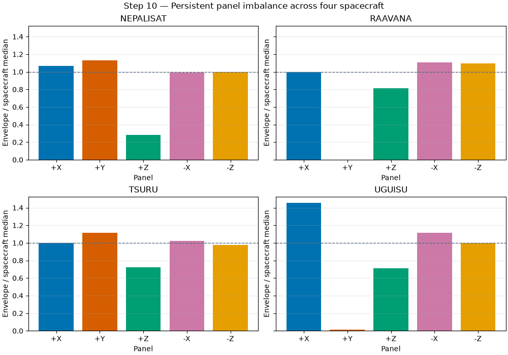
Cross-panel upper-envelope comparison (each spacecraft considered separately)
satellite panel_id  typical_p95_w  relative_to_spacecraft_median
NEPALISAT       +X       1.290905                       1.069437
NEPALISAT       +Y       1.366594                       1.132142
NEPALISAT       +Z       0.341799                       0.283160
NEPALISAT       -X       1.194164                       0.989293
NEPALISAT       -Z       1.207088                       1.000000
  RAAVANA       +X       1.319676                       1.000000
  RAAVANA       +Y       0.000036                       0.000027
  RAAVANA       +Z       1.074752                       0.814406
  RAAVANA       -X       1.463455                       1.108950
  RAAVANA       -Z       1.442462                       1.093042
    TSURU       +X       1.106144                       1.000000
    TSURU       +Y       1.233549                       1.115179
    TSURU       +Z       0.800545                       0.723726
    TSURU       -X       1.132024                       1.023396
    TSURU       -Z       1.080510                       0.976826
   UGUISU       +X       1.705784                       1.452762
   UGUISU       +Y       0.013357                       0.011376
   UGUISU       +Z       0.833557                       0.709914
   UGUISU       -X       1.310974                       1.116515
   UGUISU       -Z       1.174166                       1.000000
The detailed plots now resolve thousands of genuine timestamps within the available recordings, while TSURU adds 40 campaign-level comparison points. Sparse campaign coverage must not be treated as continuous mission history: do not integrate across missing dates or infer a mission energy yield. Precisely timed ephemeris, attitude and calibrated illumination data would be needed before these descriptive comparisons become physical diagnostics.
Total running time of the script: (0 minutes 9.824 seconds)