Note
Go to the end to download the full example code.
Real ISS elements: position, ground track and eclipse#
This reproducible example uses a historical CelesTrak OMM reproduced in the official Skyfield guide. It runs near the pinned May 2024 epoch, not at the current time. The live web view uses the same propagation helper with current cached orbital elements. See Live satellite tracking for the live application, API, provider policies and accuracy limits.
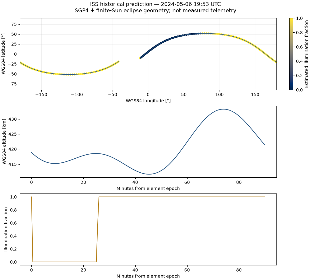
181 states; inertial speed 7651-7669 m/s
import json
from datetime import timedelta
from pathlib import Path

import matplotlib.pyplot as plt
import numpy as np

import orbitalpv as opv

start = Path(globals().get("__file__", Path.cwd())).resolve()
root = next(p for p in [start, *start.parents] if (p / "pyproject.toml").exists())
omm = json.loads((root / "examples/data/iss_omm.json").read_text())
epoch = opv.omm_epoch(omm)
times = [epoch + timedelta(seconds=i) for i in range(0, 5401, 30)]
states = opv.propagate_ground_track(omm, times)
lon = np.array([s.longitude_deg for s in states])
lat = np.array([s.latitude_deg for s in states])
altitude = np.array([s.altitude_m for s in states]) / 1000
illumination = np.array([s.illumination_fraction for s in states])
minutes = np.arange(len(states)) / 2

fig, axes = plt.subplots(3, 1, figsize=(10, 9), layout="constrained")
# NaN breaks prevent an artificial line through Greenwich at the antimeridian.
breaks = np.flatnonzero(np.abs(np.diff(lon)) > 180) + 1
axes[0].plot(np.insert(lon, breaks, np.nan), np.insert(lat, breaks, np.nan), color="#245482", lw=1)
scatter = axes[0].scatter(lon, lat, c=illumination, cmap="cividis", vmin=0, vmax=1, s=14)
fig.colorbar(scatter, ax=axes[0], label="Estimated illumination fraction")
axes[0].set(
    xlim=(-180, 180), ylim=(-90, 90), xlabel="WGS84 longitude [°]", ylabel="WGS84 latitude [°]"
)
axes[0].grid(alpha=0.2)
axes[1].plot(minutes, altitude, color="#245482")
axes[1].set(ylabel="WGS84 altitude [km]", xlabel="Minutes from element epoch")
axes[2].plot(minutes, illumination, color="#b27c13")
axes[2].set(ylabel="Illumination fraction", ylim=(-0.05, 1.05), xlabel="Minutes from element epoch")
fig.suptitle(
    f"ISS historical prediction — {epoch:%Y-%m-%d %H:%M} UTC\nSGP4 + finite-Sun eclipse geometry; not measured telemetry"
)
print(
    f"{len(states)} states; inertial speed {min(s.speed_m_s for s in states):.0f}-{max(s.speed_m_s for s in states):.0f} m/s"
)
plt.show()
Total running time of the script: (0 minutes 1.245 seconds)