Note
Go to the end to download the full example code.
Detect PV footprints in an unseen satellite image#
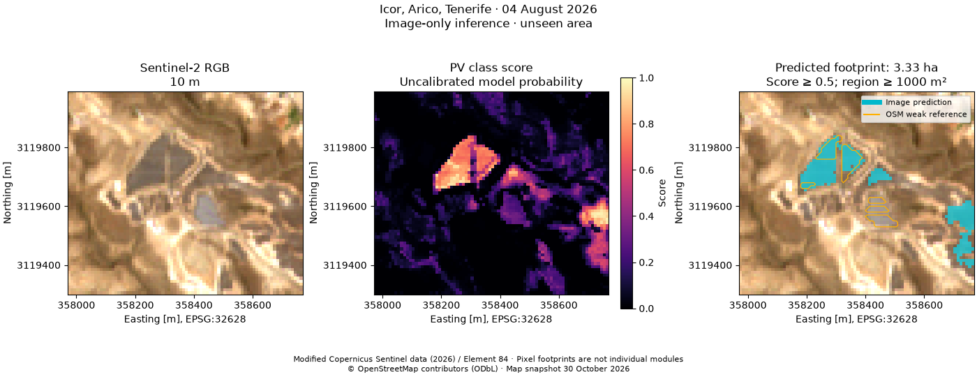
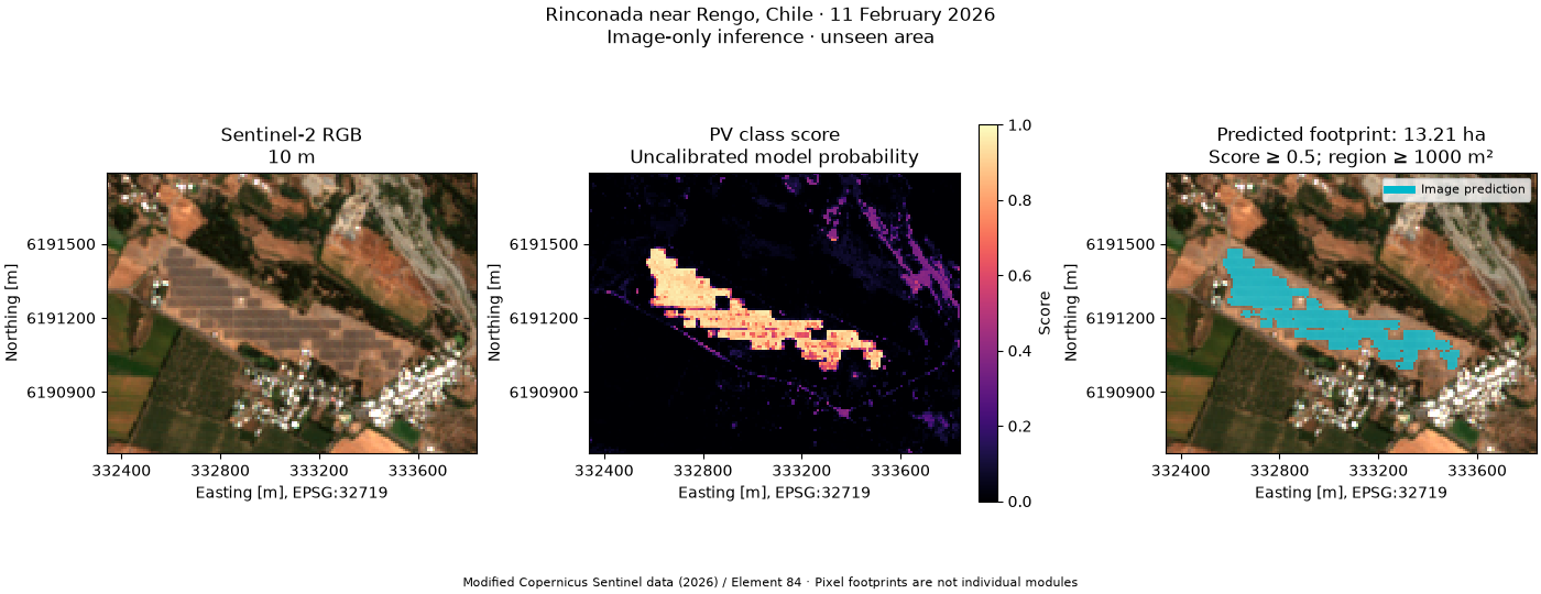
Train a small, reproducible spectral classifier on Cestas, France and apply it to Icor, Tenerife, without giving the detector Tenerife’s OSM features. Predict Rinconada, Chile with the same unchanged model.
The output is an image-derived candidate mask and GeoJSON footprint, not a copy of the map outlines. Six calibrated Sentinel-2 bands and three spectral indices drive the classifier. The default threshold (0.5) and connected-area filter (1,000 m²) are fixed before inspecting the held-out site.
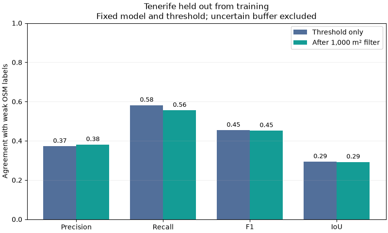
Cestas’s mapped generator polygons supply weak positive labels. Background negatives are an explicit assumption, and a 20 m outside buffer is left unknown. Tenerife’s later OSM snapshot is used only for evaluation and orange reference outlines. Its fine array rows and 10 m image pixels describe different spatial detail. These scores measure agreement with weak map labels; they do not establish surveyed or worldwide accuracy.
The example exposes modest cross-site transfer: false positives and missed arrays remain visible. Rinconada has only a mapped whole-plant boundary, so we do not score that perimeter as panel-level ground truth. More diverse, independently labelled training sites are needed for operational deployment.
Install orbital-pv[ground,examples] from this repository and keep the
companion _data directory when running this script. All imagery and labels
are real, fixed snapshots; the example runs offline. Contains modified
Copernicus Sentinel data / Element 84 and © OpenStreetMap contributors, ODbL.
directory = Path(__file__).resolve().parent if "__file__" in globals() else Path.cwd()
data = directory / "_data"
config = json.loads((data / "pv-sites.json").read_text())
sites = {
    name: opv.load_pv_site(
        **settings,
        cache_dir=data,
        offline=True,
        assets=("visual", "scl", *opv.PV_SPECTRAL_BANDS),
    )
    for name, settings in config.items()
}
training = opv.prepare_pv_training_sample(
    sites["cestas"],
    site_id="cestas",
    background_is_negative=True,
)
model = opv.PVFootprintModel.fit([training], random_state=0)
features = opv.build_pv_features(sites["tenerife"].images)
prediction = model.predict(features, threshold=0.5, min_area_m2=1000)

# The separate reference is created after inference, for comparison only.
reference = opv.prepare_pv_training_sample(
    sites["tenerife"],
    site_id="tenerife",
    background_is_negative=True,
)
opv.plot_pv_detection(
    sites["tenerife"],
    prediction,
    reference_labels=reference.labels,
    reference_label="OSM weak reference",
    reference_credit="© OpenStreetMap contributors (ODbL) · Map snapshot 30 October 2026",
)
plt.show()
Precision, recall, F1 and IoU expose errors that a background-dominated accuracy score can hide. Area filtering is reported separately.
metrics = model.evaluate(
    features,
    reference.labels,
    site_id=reference.site_id,
    label_source=reference.label_source,
    threshold=0.5,
    min_area_m2=1000,
)
pprint(metrics, sort_dicts=False)
names = ("precision", "recall", "f1", "iou")
x = np.arange(len(names))
fig, ax = plt.subplots(figsize=(8, 4.8), layout="constrained")
for shift, key, label, color in (
    (-0.19, "raw_threshold", "Threshold only", "#526f9a"),
    (0.19, "area_filtered", "After 1,000 m² filter", "#149c95"),
):
    bars = ax.bar(x + shift, [metrics[key][name] for name in names], 0.38, label=label, color=color)
    ax.bar_label(bars, fmt="%.2f", padding=3, fontsize=9)
ax.set(
    xticks=x,
    xticklabels=("Precision", "Recall", "F1", "IoU"),
    ylim=(0, 1),
    ylabel="Agreement with weak OSM labels",
    title="Tenerife held out from training\nFixed model and threshold; uncertain buffer excluded",
)
ax.legend(loc="upper right")
ax.grid(axis="y", alpha=0.2)
plt.show()
{'site_id': 'tenerife',
 'scene_id': 'S2A_T28RCS_20260804T115232_L2A',
 'label_source': 'OSM photovoltaic generator polygons; map snapshot '
                 '2026-10-30T10:23:04Z; image S2A_T28RCS_20260804T115232_L2A; '
                 'pixel-centre weak labels; outside boundary buffer 20 m; '
                 'background_is_negative=True; explicit_negative_polygons=0; '
                 'not independently surveyed ground truth',
 'spatially_disjoint_from_training': True,
 'model_id': '0c6400c0f50d43c5376c35f2dc86add777560a3e294acc3dbf075c0103f255fb',
 'threshold': 0.5,
 'min_area_m2': 1000,
 'raw_threshold': {'true_positive': 89,
                   'false_positive': 150,
                   'false_negative': 64,
                   'true_negative': 4869,
                   'precision': 0.3723849372384937,
                   'recall': 0.5816993464052288,
                   'f1': 0.45408163265306123,
                   'iou': 0.29372937293729373,
                   'accuracy': 0.9586233565351895,
                   'evaluated_pixels': 5172,
                   'labelled_pixels': 5172,
                   'prediction_valid_pixels': 5520,
                   'total_pixels': 5520,
                   'labelled_coverage': 1.0,
                   'evaluated_fraction': 0.9369565217391305},
 'area_filtered': {'true_positive': 85,
                   'false_positive': 138,
                   'false_negative': 68,
                   'true_negative': 4881,
                   'precision': 0.3811659192825112,
                   'recall': 0.5555555555555556,
                   'f1': 0.4521276595744681,
                   'iou': 0.2920962199312715,
                   'accuracy': 0.960170146945089,
                   'evaluated_pixels': 5172,
                   'labelled_pixels': 5172,
                   'prediction_valid_pixels': 5520,
                   'total_pixels': 5520,
                   'labelled_coverage': 1.0,
                   'evaluated_fraction': 0.9369565217391305}}
chile_prediction = model.predict(opv.build_pv_features(sites["rengo"].images))
opv.plot_pv_detection(sites["rengo"], chile_prediction)
plt.show()

# The analysis/ground_pv_mapping entry point exports these GeoJSON polygons,
# native-grid score/mask GeoTIFFs, model JSON and complete evaluation reports.
Total running time of the script: (0 minutes 3.677 seconds)