Note
Go to the end to download the full example code.
GEO weather imagers: surface-irradiance coverage and spacecraft solar power#
Model a selected five-spacecraft geostationary imaging network using the
public orbitalpv API. GEO weather imagers measure reflected sunlight and
thermal radiance. Those observations support retrieved cloud properties and
retrieved solar irradiance at Earth’s surface, such as NOAA’s ABI
downward-shortwave radiation product. They are not direct surface pyranometers
or the incoming solar-irradiance instruments used in the TSIS/SORCE examples.
The example connects two distinct questions: which ground regions have a useful viewing geometry, and how Earth eclipses affect the spacecraft’s own illustrative solar-array generation. It does not retrieve satellite images or calculate a surface-irradiance product.
Frozen nominal slot snapshot#
The following operational identities and nominal slots were checked against the operator sources on 30 October 2026. These fixed inputs make the example reproducible; they are not propagated live ephemerides or a complete inventory of weather satellites.
Spacecraft |
Longitude |
Imager |
Selected role |
|---|---|---|---|
GOES-18 |
137.0 W |
ABI |
GOES-West |
GOES-19 |
75.2 W |
ABI |
GOES-East |
Meteosat-12 |
0.0 |
FCI |
Europe/Africa full disk |
Meteosat-9 |
45.5 E |
SEVIRI |
Indian Ocean coverage |
Himawari-9 |
140.7 E |
AHI |
East Asia/western Pacific |
Meteosat-12 uses EUMETSAT’s rounded nominal 0-degree service slot; this does not specify its instantaneous station-keeping longitude. Backup and rapid-scan spacecraft are outside this selected network.
Sources#
NOAA spacecraft status and reported longitudes: https://ospo.noaa.gov/operations/goes/status.html.
EUMETSAT Meteosat-12 identity and nominal slot: https://www.eumetsat.int/our-satellites/meteosat-series.
EUMETSAT Meteosat-9 IODC slot and the MSG service’s 10-degree elevation criterion: https://www.eumetsat.int/msg-services.
JMA Himawari-9 role and longitude: https://www.jma.go.jp/jma/jma-eng/satellite/.
NOAA ABI surface-shortwave retrieval and its radiance-based processing: https://www.ncei.noaa.gov/metadata/geoportal/rest/metadata/item/gov.noaa.ncdc%3AC01524/html.
Assumptions#
The model uses a spherical Earth, circular equatorial orbits, and a 10-degree minimum ground elevation angle. Visibility is a geometric screening mask, not guaranteed imagery or irradiance-product availability. Instrument scan limits, pixel resolution, clouds, daylight and product-quality masks require separate treatment. The polar gap remains visible even with several GEO slots.
For the power comparison every spacecraft is assigned the same assumed 5 kW beginning-of-life array reference at 1361 W/m² and 25°C, ideal Sun tracking, 45°C cell temperature and a 0.96 optical factor. These are design assumptions, not the missions’ actual electrical specifications. Batteries, loads and service outages are not simulated; an array eclipse does not imply an interruption of imaging.
No network access or orbit-data downloads are needed to run this example.
from __future__ import annotations

import matplotlib.dates as mdates
import matplotlib.patheffects as path_effects
import matplotlib.pyplot as plt
import numpy as np
import pandas as pd
from matplotlib.colors import BoundaryNorm, ListedColormap
from matplotlib.lines import Line2D
from matplotlib.patches import Circle

import orbitalpv as opv
The synchronous radius follows from mu / r³ = Earth’s rotation rate². Coordinates in this first figure are Earth-fixed, viewed from the north.
SATELLITES = (
    ("GOES-18", -137.0, "ABI", "#0072B2"),
    ("GOES-19", -75.2, "ABI", "#D55E00"),
    ("Meteosat-12", 0.0, "FCI", "#009E73"),
    ("Meteosat-9", 45.5, "SEVIRI", "#CC79A7"),
    ("Himawari-9", 140.7, "AHI", "#B58900"),
)
MINIMUM_ELEVATION_DEG = 10.0
earth_radius_m = opv.EARTH_EQUATORIAL_RADIUS_M
geo_radius_m = (
    opv.EARTH_STANDARD_GRAVITATIONAL_PARAMETER_M3_S2 / opv.EARTH_ROTATION_RATE_RAD_S**2
) ** (1.0 / 3.0)
altitude_m = geo_radius_m - earth_radius_m
longitudes_deg = np.array([satellite[1] for satellite in SATELLITES])
slots_m = opv.keplerian_orbit_positions_m(
    geo_radius_m, 0.0, 0.0, true_anomaly_rad=np.deg2rad(longitudes_deg)
)
print(f"Ideal synchronous altitude: {altitude_m / 1000:.3f} km")
print(f"Minimum geometric viewing elevation: {MINIMUM_ELEVATION_DEG:.1f} degrees")
for name, longitude, imager, _color in SATELLITES:
    print(f"{name:12s} {longitude:+7.1f} deg longitude | {imager}")

fig, ax = plt.subplots(figsize=(9, 8), layout="constrained")
ax.add_patch(Circle((0, 0), geo_radius_m / 1e6, fill=False, linestyle="--", edgecolor="#94A3B8"))
ax.add_patch(Circle((0, 0), earth_radius_m / 1e6, color="#A4CBE4", ec="#355C7D"))
ax.text(0, 0, "Earth", ha="center", va="center", fontsize=10)
for (name, longitude, _imager, color), position in zip(SATELLITES, slots_m, strict=True):
    x, y = position[:2] / 1e6
    ax.plot([0, x], [0, y], color=color, linewidth=0.8, alpha=0.5)
    ax.scatter(x, y, s=75, color=color, edgecolors="white", zorder=3)
    ax.annotate(
        f"{name}\n{longitude:+.1f}°",
        (x, y),
        xytext=(8 if x >= 0 else -8, 8 if y >= 0 else -8),
        textcoords="offset points",
        ha="left" if x >= 0 else "right",
        va="bottom" if y >= 0 else "top",
        fontsize=9,
    )
ax.set(
    xlim=(-58, 58),
    ylim=(-53, 53),
    aspect="equal",
    xlabel="Earth-fixed x [thousand km]; Greenwich is toward +x",
    ylabel="Earth-fixed y [thousand km]; 90° E is toward +y",
    title="Step 1 — Selected GEO imaging network, north-pole view",
)
ax.grid(alpha=0.2)
plt.show()
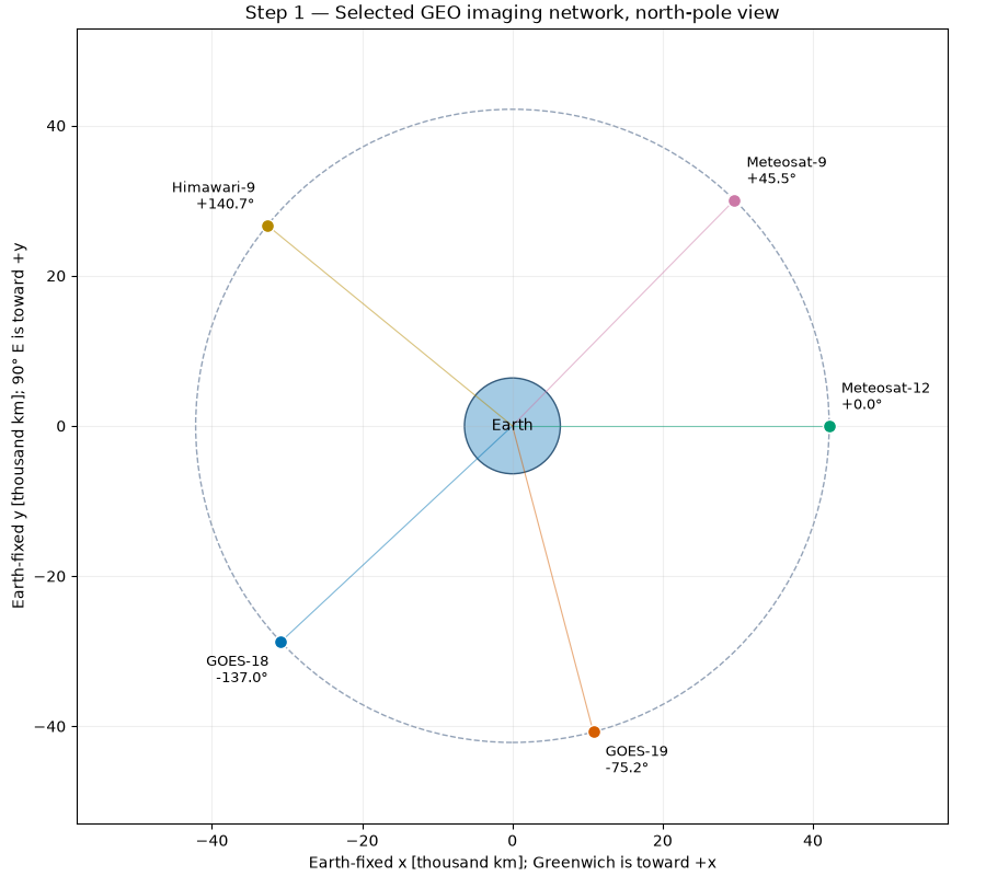
Ideal synchronous altitude: 35786.032 km
Minimum geometric viewing elevation: 10.0 degrees
GOES-18       -137.0 deg longitude | ABI
GOES-19        -75.2 deg longitude | ABI
Meteosat-12     +0.0 deg longitude | FCI
Meteosat-9     +45.5 deg longitude | SEVIRI
Himawari-9    +140.7 deg longitude | AHI
For a spherical Earth, cos(psi) = cos(latitude) cos(longitude - slot). Elevation follows from the line of sight projected onto the local vertical. The same threshold is applied to every slot as a comparison assumption. Coverage is independent of spacecraft eclipse and of the ground’s daylight.
def ground_elevation_deg(latitude_deg, longitude_deg, slot_longitude_deg):
    """Return geometric GEO elevation above a spherical local horizon."""
    cos_psi = np.cos(np.deg2rad(latitude_deg)) * np.cos(
        np.deg2rad(np.asarray(longitude_deg) - slot_longitude_deg)
    )
    slant_range_m = np.sqrt(
        geo_radius_m**2 + earth_radius_m**2 - 2 * geo_radius_m * earth_radius_m * cos_psi
    )
    sine_elevation = (geo_radius_m * cos_psi - earth_radius_m) / slant_range_m
    return np.rad2deg(np.arcsin(np.clip(sine_elevation, -1.0, 1.0)))


longitude_grid, latitude_grid = np.meshgrid(
    np.arange(-179.5, 180.0, 1.0), np.arange(-89.5, 90.0, 1.0)
)
elevation_maps = np.stack(
    [ground_elevation_deg(latitude_grid, longitude_grid, slot) for slot in longitudes_deg]
)
coverage_count = (elevation_maps >= MINIMUM_ELEVATION_DEG).sum(axis=0)
area_weights = np.cos(np.deg2rad(latitude_grid))
for threshold in (1, 2):
    fraction = np.sum(area_weights * (coverage_count >= threshold)) / np.sum(area_weights)
    print(f"Spherical surface with at least {threshold} view(s): {100 * fraction:.2f}%")

colors = ListedColormap(["#F1F3F5", "#D3E4F2", "#A5C9E3", "#6BA1CB", "#356F9F", "#143E61"])
norm = BoundaryNorm(np.arange(-0.5, len(SATELLITES) + 1.5), colors.N)
fig, ax = plt.subplots(figsize=(12, 6.2), layout="constrained")
mesh = ax.pcolormesh(longitude_grid, latitude_grid, coverage_count, cmap=colors, norm=norm)
for (_name, longitude, _imager, color), elevation in zip(SATELLITES, elevation_maps, strict=True):
    ax.contour(
        longitude_grid,
        latitude_grid,
        elevation,
        levels=[MINIMUM_ELEVATION_DEG],
        colors=[color],
        linewidths=1,
    )
    ax.scatter(longitude, 0, marker="v", s=38, color=color, edgecolors="white", zorder=5)

sites = [
    ("Boulder", -105.27, 40.01),
    ("Santiago", -70.67, -33.45),
    ("Madrid", -3.70, 40.42),
    ("Delhi", 77.21, 28.61),
    ("Tokyo", 139.69, 35.68),
    ("Sydney", 151.21, -33.87),
]
for name, longitude, latitude in sites:
    ax.scatter(longitude, latitude, marker="x", s=20, color="#242B35", zorder=6)
    annotation = ax.annotate(
        name, (longitude, latitude), xytext=(5, 5), textcoords="offset points", fontsize=8
    )
    annotation.set_path_effects([path_effects.withStroke(linewidth=2.5, foreground="white")])
ax.set(
    xlim=(-180, 180),
    ylim=(-90, 90),
    xticks=np.arange(-180, 181, 45),
    yticks=np.arange(-90, 91, 30),
    xlabel="Longitude [degrees east]",
    ylabel="Latitude [degrees north]",
    title="Step 2 — Number of available geometric views, elevation ≥ 10°",
)
ax.grid(alpha=0.2)
fig.colorbar(mesh, ax=ax, ticks=range(len(SATELLITES) + 1), label="Visible spacecraft")
ax.legend(
    handles=[
        Line2D([0], [0], color=color, label=name) for name, _lon, _imager, color in SATELLITES
    ],
    loc="upper center",
    bbox_to_anchor=(0.5, -0.16),
    ncols=3,
    fontsize=8,
    title="Colored contours: each spacecraft's 10° elevation boundary",
)
plt.show()
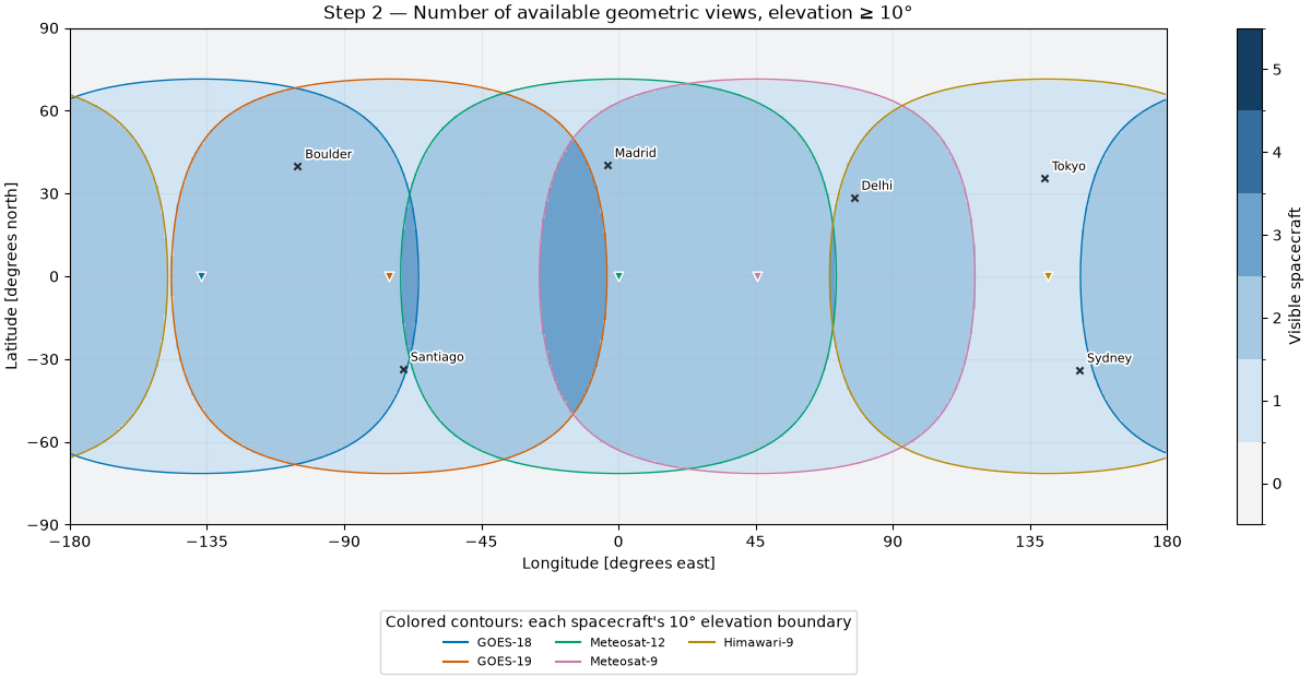
Spherical surface with at least 1 view(s): 93.69%
Spherical surface with at least 2 view(s): 72.39%
This is an idealized equinox day. At t=0 the Sun is over Greenwich at local solar noon; the horizontal axis is elapsed mean-solar time, not a claimed UTC prediction. Earth rotates at the sidereal rate while the idealized Sun advances at their difference, giving a 24-hour solar day. The Sun is at zero declination and one AU; finite solar-disc overlap includes penumbra. Arrays track the Sun perfectly and every satellite uses the stated 5 kW reference. Independent spacecraft cannot share the plotted aggregate power.
time_s = np.arange(0.0, 86_400.0 + 30.0, 30.0)
earth_angle = opv.EARTH_ROTATION_RATE_RAD_S * time_s
sun_angle = (opv.EARTH_ROTATION_RATE_RAD_S - 2 * np.pi / 86_400.0) * time_s
sun_positions_m = opv.ASTRONOMICAL_UNIT_M * np.column_stack(
    [np.cos(sun_angle), np.sin(sun_angle), np.zeros_like(sun_angle)]
)
reference = opv.PvwattsReference(
    pdc0_w=5_000.0,
    gamma_pdc_per_c=-0.002,
    reference_irradiance_w_m2=1361.0,
    reference_temperature_c=25.0,
)
power_w = np.empty((len(time_s), len(SATELLITES)))
for index, (_name, longitude, _imager, _color) in enumerate(SATELLITES):
    positions_m = opv.keplerian_orbit_positions_m(
        geo_radius_m, 0.0, 0.0, true_anomaly_rad=earth_angle + np.deg2rad(longitude)
    )
    illumination = np.array(
        [
            opv.earth_occultation_fraction(position, sun)
            for position, sun in zip(positions_m, sun_positions_m, strict=True)
        ]
    )
    solar_distance_m = np.linalg.norm(sun_positions_m - positions_m, axis=1)
    irradiance = opv.effective_irradiance_w_m2(
        opv.am0_irradiance(solar_distance_m),
        illumination,
        np.ones_like(illumination),
        optical_factor=0.96,
    )
    power_w[:, index] = opv.pvwatts_dc_space(irradiance, 45.0, reference)

fig, axes = plt.subplots(2, 1, figsize=(11, 7), sharex=True, layout="constrained")
for index, (name, _longitude, _imager, color) in enumerate(SATELLITES):
    axes[0].plot(time_s / 3600, power_w[:, index] / 1000, label=name, color=color)
axes[0].set(
    ylabel="Modelled array DC [kW]",
    title="Step 3 — Ideal equinox generation; assumed 5 kW reference per spacecraft",
)
axes[0].legend(loc="upper left", bbox_to_anchor=(1.01, 1), fontsize=8)
axes[1].plot(time_s / 3600, power_w.sum(axis=1) / 1000, color="#243B53")
axes[1].set(
    xlabel="Hours since Greenwich local solar noon (idealized day)",
    ylabel="Modelled sum [kW]",
    xticks=np.arange(0, 25, 3),
    xlim=(0, 24),
)
for ax in axes:
    ax.grid(alpha=0.25)
plt.show()

energy_kwh = np.asarray(np.trapezoid(power_w, time_s, axis=0)) / 3.6e6
for (name, _longitude, _imager, _color), energy in zip(SATELLITES, energy_kwh, strict=True):
    print(f"Illustrative equinox array energy, {name}: {energy:.2f} kWh/day")
print(f"Minimum aggregate illustrative array power: {power_w.sum(axis=1).min() / 1000:.2f} kW")
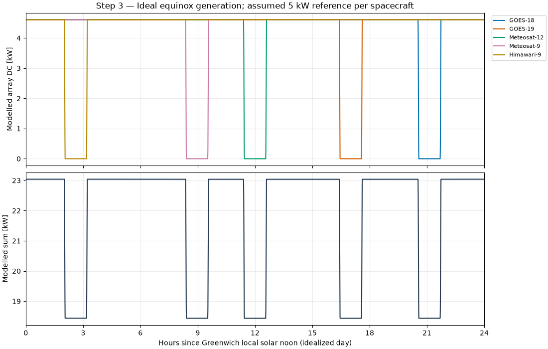
Illustrative equinox array energy, GOES-18: 105.25 kWh/day
Illustrative equinox array energy, GOES-19: 105.25 kWh/day
Illustrative equinox array energy, Meteosat-12: 105.25 kWh/day
Illustrative equinox array energy, Meteosat-9: 105.25 kWh/day
Illustrative equinox array energy, Himawari-9: 105.25 kWh/day
Minimum aggregate illustrative array power: 18.43 kW
A circular equatorial GEO orbit has beta angle equal to the solar declination. A simple sinusoidal 365-day declination model illustrates the seasons; it is not a date-specific ephemeris. The reusable cylindrical-shadow helper neglects penumbra, Earth oblateness and the atmosphere. All five slots have essentially the same seasonal duration, but longitude shifts the time of day at which the eclipse occurs, as the previous figure demonstrates.
dates = pd.date_range("2026-01-01", periods=365, freq="D", tz="UTC")
day_of_year = np.arange(1, 366)
declination_deg = 23.44 * np.sin(2 * np.pi * (day_of_year - 80) / 365.0)
eclipse_minutes = np.array(
    [opv.circular_eclipse_duration_s(altitude_m, beta) / 60 for beta in declination_deg]
)
fig, ax = plt.subplots(figsize=(10, 4.8), layout="constrained")
ax.plot(dates, eclipse_minutes, color="#243B53", label="Cylindrical-shadow duration per orbit")
ax.fill_between(dates, eclipse_minutes, color="#A5C9E3", alpha=0.7)
ax.set(
    xlabel="Month in schematic annual cycle (2026 calendar labels)",
    ylabel="Modelled eclipse duration [minutes/orbit]",
    title="Step 4 — GEO eclipse seasons; same ideal duration at all five slots",
    ylim=(0, 80),
)
ax.xaxis.set_major_locator(mdates.MonthLocator())
ax.xaxis.set_major_formatter(mdates.DateFormatter("%b"))
ax.grid(alpha=0.25)
ax.legend(loc="upper right", fontsize=8)
plt.show()
print(f"Peak cylindrical-shadow duration: {eclipse_minutes.max():.2f} min/orbit")
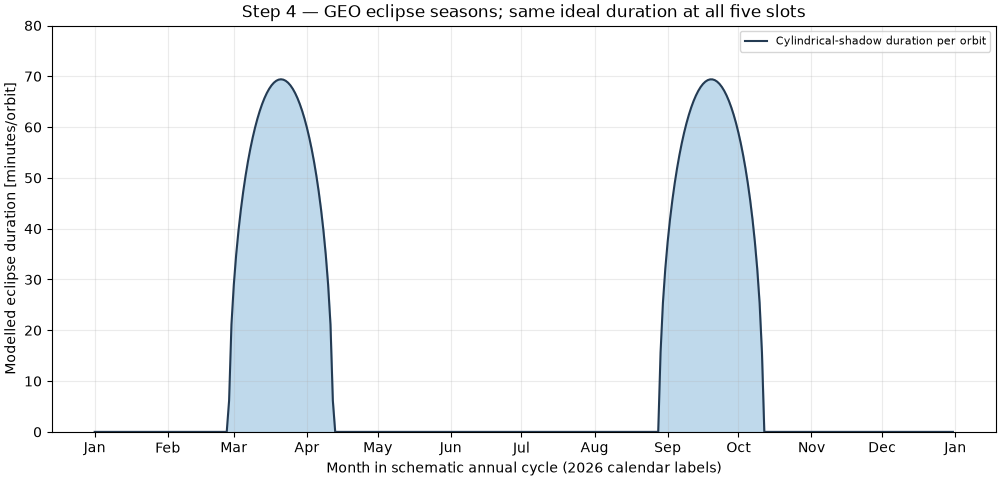
Peak cylindrical-shadow duration: 69.41 min/orbit
GEO imaging offers persistent regional viewing geometry and overlap between some slots, while high latitudes remain poorly served. A surface-radiation retrieval still requires calibrated imagery, cloud/atmospheric inputs and product-specific quality screening. The separate PV calculation explains why spacecraft electrical design must accommodate seasonal eclipses; it does not predict the delivered irradiance product or mission availability.
Total running time of the script: (0 minutes 1.126 seconds)