Note
Go to the end to download the full example code.
Flying Laptop: a month of measured solar-array generation#
Use the public orbitalpv API to download calibrated, real on-orbit voltage
and current measurements from the University of Stuttgart’s Flying Laptop
satellite. February 2018 contains 75,097 packet timestamps and 300,388
array observations across right, left, center and experimental test arrays.
Install pip install "orbital-pv[examples]". The first run downloads one
30 MB compressed monthly archive; subsequent runs reuse it. The connector
reads only electrical packet 4900 inside the archive without extracting files
to disk. No interpolation or synthetic records are added.
Source and interpretation#
FLP Team (2019), FLP Telemetry Data, DaRUS, CC BY 4.0: https://doi.org/10.18419/darus-451.
Official units and packet definitions: https://doi.org/10.18419/darus-456.
Selected archive: https://darus.uni-stuttgart.de/api/access/datafile/264.
The source timestamps are UTC packet-generation times, expressed as Unix epoch milliseconds. They are not radio reception times. The official data description allows up to 400 ms between sensor acquisition and packet timing. The packet supplies calibrated voltages in V and currents in A; electrical power below is computed as their product rather than independently measured.
The test channel is an experimental array channel aboard the spacecraft,
not a ground-test session. Small signed sensor offsets are retained. Recorded
values describe the operating system and do not, by themselves, establish
maximum-power capability, irradiance-normalized efficiency or degradation.
from __future__ import annotations

from pathlib import Path
from tempfile import gettempdir

import matplotlib.dates as mdates
import matplotlib.pyplot as plt
import pandas as pd

import orbitalpv as opv
The local loader verifies the download’s checksum sidecar when present. Every packet contributes four array observations. Missing values are omitted per voltage/current pair rather than replaced with zeros.
cache = Path(gettempdir()) / "orbitalpv-real-data"
archive = cache / "FLP_TM_HK_2018-02.tar.bz2"
if archive.exists():
    telemetry = opv.load_flying_laptop_power(archive)
else:
    telemetry = opv.fetch_flying_laptop_power("2018-02", archive)

times = telemetry["timestamp"].drop_duplicates().sort_values()
gaps = times.diff().dt.total_seconds()
print(f"Packet timestamps: {len(times):,}")
print(f"Array observations: {len(telemetry):,}")
print(f"UTC packet coverage: {times.min()} to {times.max()}")
print(f"Median interval: {gaps.median():.3f} s; largest gap: {gaps.max():.3f} s")
print(f"Source DOI: {telemetry.attrs['dataset_doi']}")
print(f"Archive SHA256: {telemetry.attrs['sha256']}")

daily_counts = times.groupby(times.dt.floor("D")).size()
fig, ax = plt.subplots(figsize=(10, 4), layout="constrained")
ax.bar(daily_counts.index, daily_counts.values, width=0.8, color="#586A83")
ax.set(
    title="Step 1 — Recorded Flying Laptop packets per day",
    xlabel="UTC date",
    ylabel="Unique packet timestamps",
)
ax.xaxis.set_major_locator(mdates.DayLocator(interval=4))
ax.xaxis.set_major_formatter(mdates.DateFormatter("%d %b"))
ax.grid(True, axis="y", alpha=0.25)
plt.show()
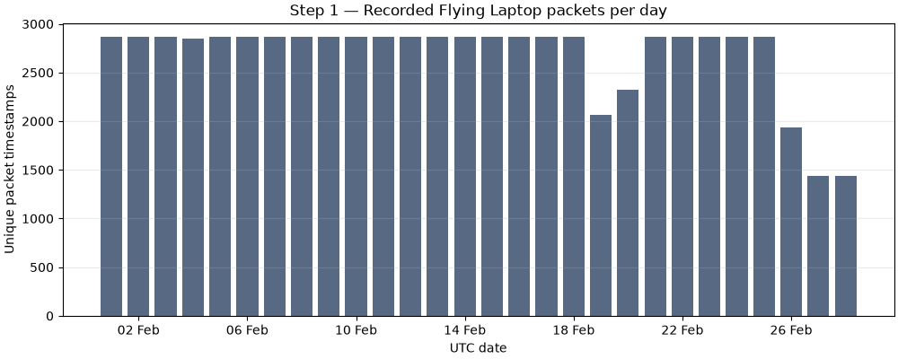
Packet timestamps: 75,097
Array observations: 300,388
UTC packet coverage: 2018-02-01 00:00:11.952000+00:00 to 2018-02-28 23:59:25.624000+00:00
Median interval: 30.150 s; largest gap: 663.300 s
Source DOI: 10.18419/darus-451
Archive SHA256: 9ec01cfc3128cc4dad522df14cb4aa73191748791a8677e181e4ed4c6e2af1bb
All samples in this interval are displayed; discrete markers avoid drawing invented values across telemetry gaps. Array identities come from the official packet-4900 definitions, rather than inferred column positions.
start = times.min().normalize()
stop = start + pd.Timedelta(hours=6)
detail = telemetry[(telemetry["timestamp"] >= start) & (telemetry["timestamp"] < stop)]
colors = {"right": "#0072B2", "left": "#D55E00", "center": "#009E73", "test": "#CC79A7"}
print(f"Detailed interval: {start} to {stop} (end excluded)")
print(f"Detailed native packet timestamps: {detail['timestamp'].nunique():,}")


def plot_native(column: str, ylabel: str, title: str) -> None:
    """Plot every supplied observation in the selected recording interval."""
    _fig, ax = plt.subplots(figsize=(10, 4.3), layout="constrained")
    for panel_id, panel in detail.groupby("panel_id", sort=True):
        ax.plot(
            panel["timestamp"],
            panel[column],
            ".",
            ms=2.5,
            alpha=0.7,
            color=colors[str(panel_id)],
            label=str(panel_id),
        )
    ax.set(title=title, xlabel="UTC packet time on 1 February 2018", ylabel=ylabel)
    ax.xaxis.set_major_locator(mdates.HourLocator())
    ax.xaxis.set_major_formatter(mdates.DateFormatter("%H:%M"))
    ax.grid(True, alpha=0.25)
    ax.legend(title="Array", loc="upper left", bbox_to_anchor=(1.01, 1))
    plt.show()


plot_native("voltage_v", "Measured array voltage [V]", "Step 2 — Calibrated array voltages")
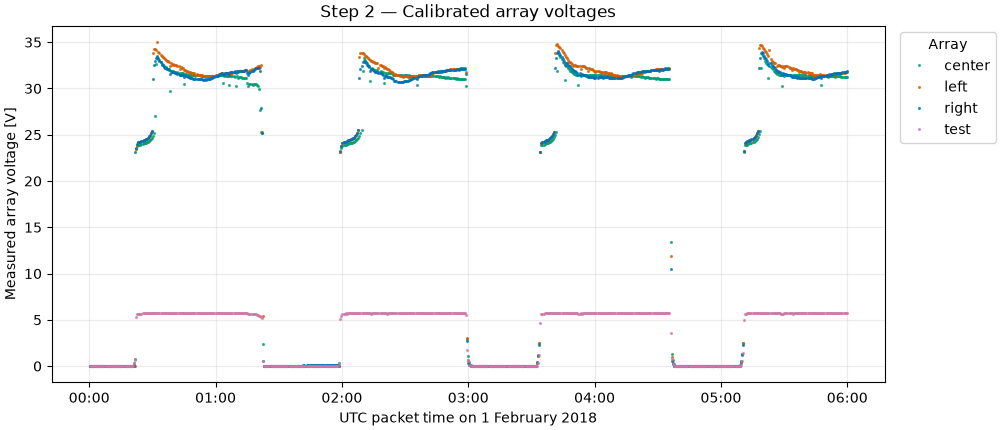
Detailed interval: 2018-02-01 00:00:00+00:00 to 2018-02-01 06:00:00+00:00 (end excluded)
Detailed native packet timestamps: 717
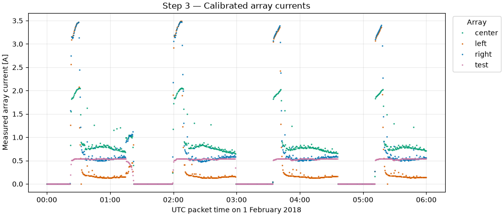
Array currents are already in amperes. Low-current periods remain part of the record; they are not automatically labeled as eclipses or faults.
plot_native("current_a", "Measured array current [A]", "Step 3 — Calibrated array currents")
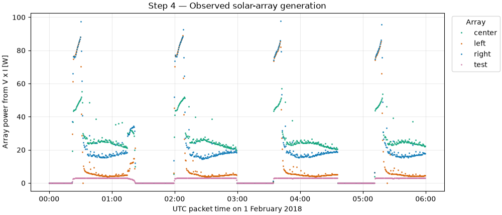
The connector computes power_w = voltage_v * current_a in each packet.
Current and voltage belong to the same array and housekeeping packet; no
nearest-neighbor matching across different telemetry streams is needed.
plot_native("power_w", "Array power from V x I [W]", "Step 4 — Observed solar-array generation")
Daily P95 values use all available observations and summarize operating behavior, including changing illumination, attitude and power-system state. They are not a degradation estimate. Coverage varies, so the counts in the first figure should be considered alongside these daily summaries.
daily = (
    telemetry.assign(day=telemetry["timestamp"].dt.floor("D"))
    .groupby(["panel_id", "day"], as_index=False)
    .agg(power_p95_w=("power_w", lambda values: float(values.quantile(0.95))))
)
fig, ax = plt.subplots(figsize=(10, 4.3), layout="constrained")
for panel_id, panel in daily.groupby("panel_id", sort=True):
    ax.scatter(
        panel["day"], panel["power_p95_w"], s=25, color=colors[str(panel_id)], label=str(panel_id)
    )
ax.set(
    title="Step 5 — Daily P95 of observed array power",
    xlabel="UTC date",
    ylabel="Daily 95th-percentile power [W]",
)
ax.xaxis.set_major_locator(mdates.DayLocator(interval=4))
ax.xaxis.set_major_formatter(mdates.DateFormatter("%d %b"))
ax.grid(True, alpha=0.25)
ax.legend(title="Array", loc="upper left", bbox_to_anchor=(1.01, 1))
plt.show()
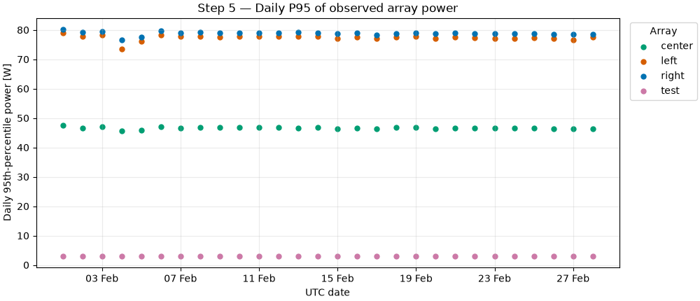
This dataset adds a month-scale history of genuine spacecraft electrical measurements, with recorded gaps. Use the full connector time filters to select other intervals. Before interpreting changes as physical degradation, add independently verified geometry, attitude, irradiance and operating-state information. Do not integrate straight across data gaps to claim a complete mission energy yield.
Total running time of the script: (0 minutes 5.716 seconds)