Note
Go to the end to download the full example code.
Repaired panel power: accept or measure again?#
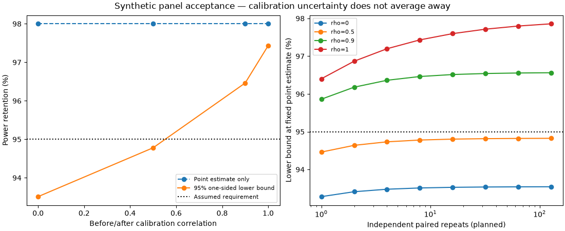
ESA’s November 5, 2026 Da Vinci report motivates electrical acceptance after panel damage. ESA publishes no numerical power data. All eight paired Pmax readings and uncertainty budgets here are synthetic assumptions, not Da Vinci measurements. A bound below the assumed 95% retention requirement means insufficient evidence, not a failed panel. Flight qualification is separate.
calibration_correlation  observations  retention  lower_retention  minimum_retention  confidence  repeat_mean_log_sigma  differential_calibration_log_sigma  combined_log_sigma  point_estimate_accepted  accepted
                    0.0             8   0.980001         0.935114               0.95        0.95               0.003536                            0.028284            0.028504                     True     False
                    0.5             8   0.980001         0.947803               0.95        0.95               0.003536                            0.020000            0.020310                     True     False
                    0.9             8   0.980001         0.964620               0.95        0.95               0.003536                            0.008944            0.009618                     True      True
                    1.0             8   0.980001         0.974319               0.95        0.95               0.003536                            0.000000            0.003536                     True      True
from dataclasses import asdict
from pathlib import Path

import matplotlib.pyplot as plt
import pandas as pd

from orbitalpv.acceptance import plan_power_retention_test, power_retention_acceptance
from orbitalpv.data import load_table

CONFIG = {
    "repeat_log_sigma": 0.01,
    "before_calibration_log_sigma": 0.02,
    "after_calibration_log_sigma": 0.02,
    "minimum_retention": 0.95,
    "confidence": 0.95,
}


def study() -> tuple[pd.DataFrame, pd.DataFrame]:
    directory = Path(__file__).resolve().parent if "__file__" in globals() else Path.cwd()
    pairs = load_table(directory / "_data/panel_acceptance.csv")
    cases = []
    for rho in (0.0, 0.5, 0.9, 1.0):
        result = power_retention_acceptance(
            pairs.before_power_w,
            pairs.after_power_w,
            calibration_correlation=rho,
            **CONFIG,
        )
        cases.append({"calibration_correlation": rho, **asdict(result)})
    plans = []
    for rho in (0.0, 0.5, 0.9, 1.0):
        for n in (1, 2, 4, 8, 16, 32, 64, 128):
            result = plan_power_retention_test(
                cases[0]["retention"], n, calibration_correlation=rho, **CONFIG
            )
            plans.append({"calibration_correlation": rho, **asdict(result)})
    return pd.DataFrame(cases), pd.DataFrame(plans)


def plot_study(cases: pd.DataFrame, plans: pd.DataFrame) -> plt.Figure:
    fig, axes = plt.subplots(1, 2, figsize=(11, 4.5), layout="constrained")
    rho = cases.calibration_correlation
    axes[0].plot(rho, 100 * cases.retention, "o--", label="Point estimate only")
    axes[0].plot(rho, 100 * cases.lower_retention, "o-", label="95% one-sided lower bound")
    axes[0].axhline(95, color="black", linestyle=":", label="Assumed requirement")
    axes[0].set(xlabel="Before/after calibration correlation", ylabel="Power retention (%)")
    axes[0].legend(fontsize=8)
    for correlation, group in plans.groupby("calibration_correlation"):
        axes[1].plot(
            group.observations, 100 * group.lower_retention, "o-", label=f"rho={correlation:g}"
        )
    axes[1].axhline(95, color="black", linestyle=":")
    axes[1].set(
        xlabel="Independent paired repeats (planned)",
        ylabel="Lower bound at fixed point estimate (%)",
        xscale="log",
    )
    axes[1].legend(fontsize=8)
    fig.suptitle("Synthetic panel acceptance — calibration uncertainty does not average away")
    return fig


if __name__ == "__main__":
    cases, plans = study()
    print(cases.to_string(index=False))
    plot_study(cases, plans)
    plt.show()
Total running time of the script: (0 minutes 0.242 seconds)