Note
Go to the end to download the full example code.
Real flight power forecasts and coherent uncertainty#
Three UTC days of native Flying Laptop right-array measurements are separated into training, calibration and evaluation. The forecast predicts operating V/I; it is not a healthy-power expectation or an available-MPP estimate.
The 8,599-row CC BY 4.0 snapshot is attributed and checksum verified. Windows
crossing gaps or partition boundaries are excluded. This example executes
offline. The reusable analysis and recorded metrics are under
analysis/flight_power_uncertainty.
directory = Path(__file__).resolve().parent if "__file__" in globals() else Path.cwd()
path = directory / "_data/flying_laptop_right_2018-02-01_03.csv"
provenance = json.loads(path.with_name(path.name + ".provenance.json").read_text())
if sha256(path.read_bytes()).hexdigest() != provenance["snapshot_sha256"]:
    raise ValueError("Measured snapshot checksum mismatch")
frame = pd.read_csv(path)
frame["timestamp"] = pd.to_datetime(frame["timestamp"], utc=True)
print(f"FLP Team, DOI {provenance['dataset_doi']}, CC BY 4.0; {len(frame):,} native V/I pairs")
FLP Team, DOI 10.18419/darus-451, CC BY 4.0; 8,599 native V/I pairs
The seasonal lag is an explicit 180-sample assumption (90.45 minutes), not a reconstructed orbit. Cadence continuity is required over the entire lag/ forecast span. The fairly long lag excludes many windows; counts are shown.
data = opv.make_lagged_vi_data(
    frame,
    lags=(0, 1, 2, 170, 176, 179),
    horizons=(1, 4, 10),
    cadence_s=30.15,
    cadence_tolerance_s=0.25,
)
train, calibration, evaluation = opv.chronological_forecast_split(
    data, training_stop="2018-02-02T00:00Z", calibration_stop="2018-02-03T00:00Z"
)
model = opv.fit_linear_vi_forecaster(train, ridge=1.0)
prediction = model.predict(evaluation)
print(f"Valid continuous windows: {len(data.features):,}/{data.source_windows:,}")
print(
    f"Fit / calibrate / evaluate: {len(train.features):,} / {len(calibration.features):,} / {len(evaluation.features):,}"
)

truth_w = evaluation.targets[..., 0] * evaluation.targets[..., 1]
forecasts = {
    "Persistence": opv.persistence_vi_forecast(evaluation),
    "Seasonal lag assumption": opv.seasonal_lag_vi_forecast(evaluation, period_steps=180),
    "Multivariate ridge": prediction,
}
fig, ax = plt.subplots(figsize=(9, 4.5), layout="constrained")
for name, values in forecasts.items():
    power_w = values[..., 0] * values[..., 1]
    error = np.abs(power_w - truth_w).mean(axis=0)
    ax.plot(np.array(data.horizons) * data.cadence_s / 60, error, "o-", label=name)
    print(name, "power MAE by horizon [W]:", error)
ax.set(
    xlabel="Nominal forecast horizon [minutes]",
    ylabel="Held-out operating-power MAE [W]",
    title="A more complex baseline does not win at every horizon",
)
ax.legend()
ax.grid(alpha=0.2)
plt.show()
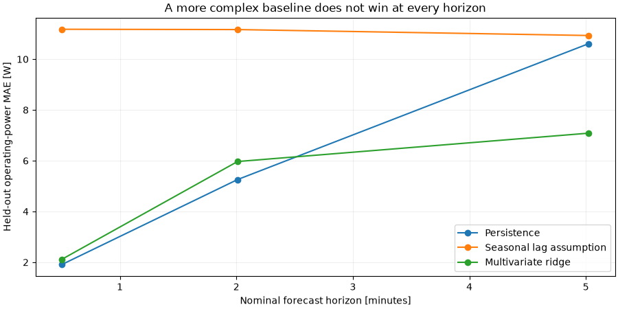
Valid continuous windows: 4,516/8,410
Fit / calibrate / evaluate: 1,395 / 1,533 / 1,578
Persistence power MAE by horizon [W]: [ 1.91058384  5.25626885 10.61191986]
Seasonal lag assumption power MAE by horizon [W]: [11.17692843 11.16547318 10.93147864]
Multivariate ridge power MAE by horizon [W]: [2.11626698 5.96700556 7.08460324]
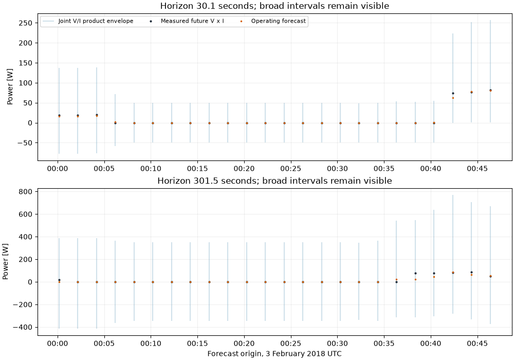
Each score is the maximum over voltage, current, all three horizons, and twenty consecutive records. Per-horizon scales use only training residuals. Power interval extrema are computed from all four rectangle corners, keeping signed telemetry possible. No independent power interval can contradict V x I.
fitted_training = model.model.predict(train.features).reshape(train.targets.shape)
scales = np.maximum((train.targets - fitted_training).std(axis=0), 1e-6)
calibrator = opv.calibrate_block_conformal_vi(
    calibration.targets,
    model.predict(calibration),
    origin_times=calibration.origin_times,
    target_end_times=calibration.target_end_times,
    trained_through=model.model.trained_through,
    scales=scales,
    coverage=0.9,
    block_size=20,
)
intervals = calibrator.predict(prediction, origin_times=evaluation.origin_times)
metrics = intervals.empirical_coverage(evaluation.targets)
print("Joint held-out coverage and widths:", metrics)
Joint held-out coverage and widths: {'joint_vi_coverage': 0.9923954372623575, 'joint_power_coverage': 0.9987325728770595, 'mean_voltage_width_v': 89.03673736695202, 'mean_current_width_a': 8.217060590411288, 'mean_power_width_w': 574.7488666905027}
This deliberately simple envelope is broad around a changing operating regime. High coverage alone does not make it useful for control. Temporal block exchangeability is an assumption, not established by chronological splitting. The recorded width exposes the need for regime-aware models. Individual vertical segments avoid joining bands across excluded gaps.
selected = np.flatnonzero(
    evaluation.origin_times < evaluation.origin_times[0] + pd.Timedelta(hours=2)
)[::4]
times = evaluation.origin_times[selected]
fig, axes = plt.subplots(2, 1, figsize=(10, 7), layout="constrained")
for index, ax in enumerate(axes):
    horizon_index = (0, 2)[index]
    ax.vlines(
        times,
        intervals.power_lower_w[selected, horizon_index],
        intervals.power_upper_w[selected, horizon_index],
        color="#7AAAC4",
        alpha=0.35,
        label="Joint V/I product envelope",
    )
    ax.plot(
        times,
        truth_w[selected, horizon_index],
        ".",
        color="#202C39",
        ms=4,
        label="Measured future V x I",
    )
    ax.plot(
        times,
        intervals.power_prediction_w[selected, horizon_index],
        ".",
        color="#D55E00",
        ms=3,
        label="Operating forecast",
    )
    ax.set(
        ylabel="Power [W]",
        title=f"Horizon {data.horizons[horizon_index] * data.cadence_s:.1f} seconds; broad intervals remain visible",
    )
    ax.xaxis.set_major_formatter(mdates.DateFormatter("%H:%M"))
    ax.grid(alpha=0.2)
axes[0].legend(loc="upper left", ncols=3, fontsize=8)
axes[-1].set_xlabel("Forecast origin, 3 February 2018 UTC")
plt.show()
Total running time of the script: (0 minutes 0.412 seconds)