Note
Go to the end to download the full example code.
Temperature and radiation sensitivity of space cells#
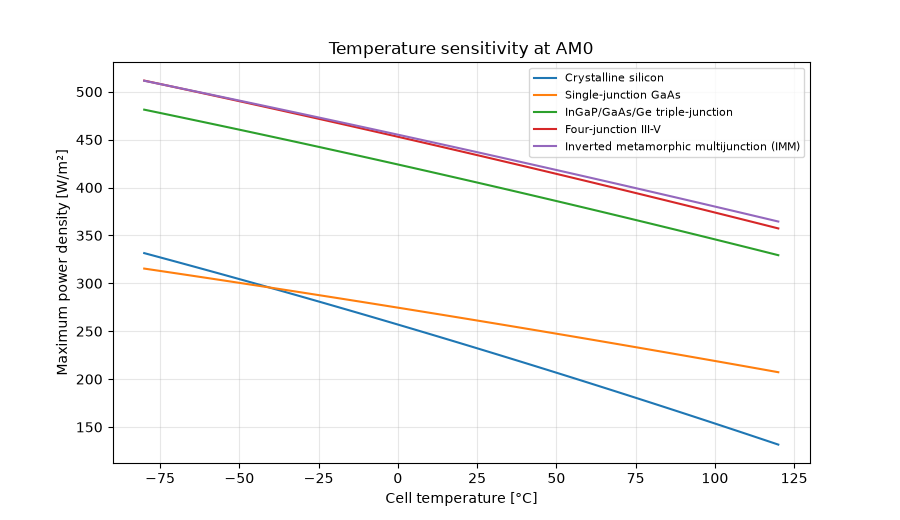
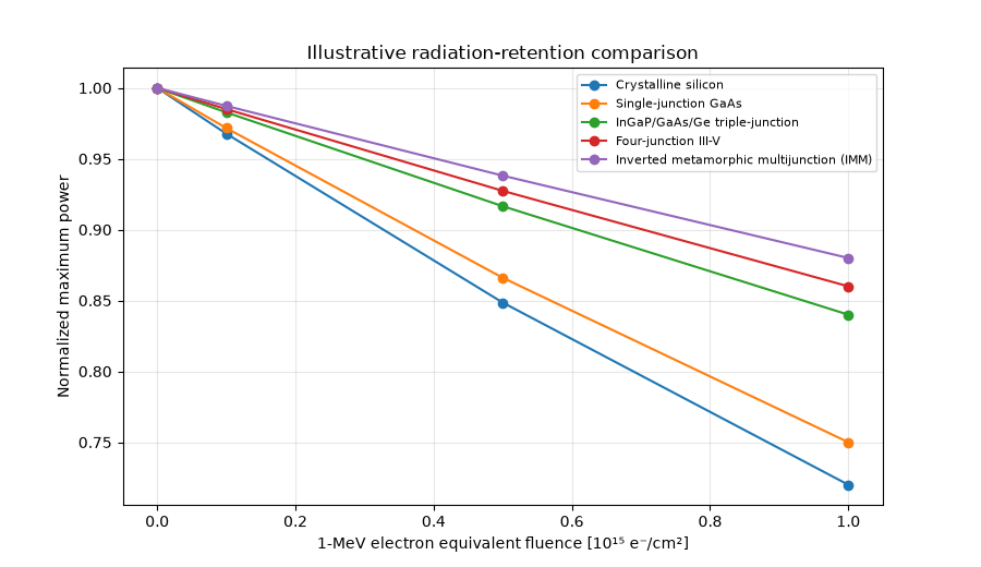
Use the public orbitalpv API to compare how representative space-cell technologies respond to cell temperature and accumulated 1-MeV-electron equivalent fluence.
The built-in radiation-retention coefficients are deliberately exposed as technology-level comparative assumptions, not manufacturer qualification data.
from __future__ import annotations

import matplotlib.pyplot as plt
import numpy as np

import orbitalpv as opv

technologies = opv.list_space_cell_technologies()
temperature_c = np.linspace(-80.0, 120.0, 81)
fluence_cases = [0.0, 1.0e14, 5.0e14, 1.0e15]

fig, ax = plt.subplots(figsize=(9, 5.2))
for technology in technologies:
    pmp = [
        opv.simulate_space_cell(
            technology,
            cell_temperature_c=float(temp_c),
        ).pmp_w_m2
        for temp_c in temperature_c
    ]
    ax.plot(temperature_c, pmp, label=technology.name)

ax.set(xlabel="Cell temperature [°C]", ylabel="Maximum power density [W/m²]")
ax.set_title("Temperature sensitivity at AM0")
ax.grid(True, alpha=0.3)
ax.legend(fontsize=8)
plt.show()

fig, ax = plt.subplots(figsize=(9, 5.2))
for technology in technologies:
    bol = opv.simulate_space_cell(technology).pmp_w_m2
    normalized_power = [
        opv.simulate_space_cell(
            technology,
            fluence_1mev_e_cm2=fluence,
        ).pmp_w_m2
        / bol
        for fluence in fluence_cases
    ]
    ax.plot(
        np.asarray(fluence_cases) / 1.0e15,
        normalized_power,
        marker="o",
        label=technology.name,
    )

ax.set(
    xlabel="1-MeV electron equivalent fluence [10¹⁵ e⁻/cm²]",
    ylabel="Normalized maximum power",
)
ax.set_title("Illustrative radiation-retention comparison")
ax.grid(True, alpha=0.3)
ax.legend(fontsize=8)
plt.show()
Total running time of the script: (0 minutes 0.218 seconds)