Note
Go to the end to download the full example code.
Follow panel temperature through sunlight and eclipse#
An illustrative two-orbit case couples a transient thermal node to temperature- dependent PV electricity. Input irradiance is already projected on the panel; the example’s 90-minute orbit and fluxes are declared synthetic assumptions.
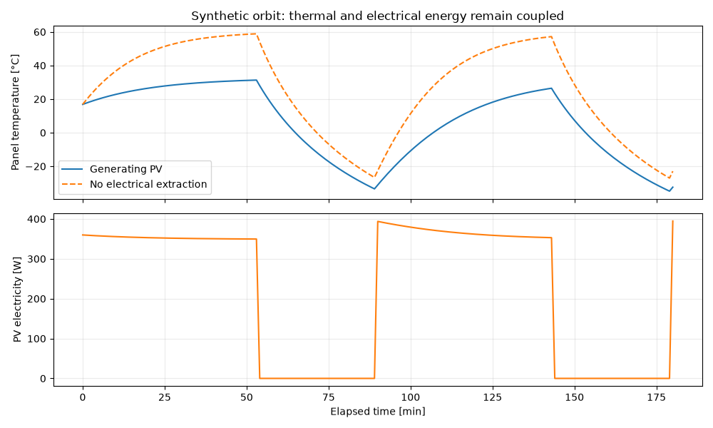
Maximum energy-balance residual: 1.86e-09 J
import matplotlib.pyplot as plt
import numpy as np

from orbitalpv import physics as opv

# Step 1: provide solar/albedo and Earth-IR fluxes separately.
time = np.arange(0.0, 10801.0, 60)
sunlight = (time % 5400) < 3240
solar = np.where(sunlight, 1100.0, 0.0)
albedo = np.where(sunlight, 80.0, 0.0)
surface = opv.ThermalSurface(area_m2=1, radiating_area_m2=2, heat_capacity_j_k=12000)

# Step 2: remove PV electrical extraction from the panel thermal balance.
model = opv.simulate_panel_thermal(
    time,
    solar,
    surface=surface,
    albedo_w_m2=albedo,
    earth_ir_w_m2=150,
    pv_efficiency=0.3,
    initial_temperature_k=290,
)
without_extraction = opv.simulate_panel_thermal(
    time,
    solar,
    surface=surface,
    albedo_w_m2=albedo,
    earth_ir_w_m2=150,
    pv_efficiency=0,
    initial_temperature_k=290,
)

# Step 3: inspect both thermal dynamics and electrical output.
fig, axes = plt.subplots(2, 1, figsize=(10, 6), sharex=True)
axes[0].plot(time / 60, model.temperature_k - 273.15, label="Generating PV")
axes[0].plot(
    time / 60,
    without_extraction.temperature_k - 273.15,
    label="No electrical extraction",
    linestyle="--",
)
axes[0].set(
    ylabel="Panel temperature [°C]",
    title="Synthetic orbit: thermal and electrical energy remain coupled",
)
axes[0].legend()
axes[1].plot(time / 60, model.pv_power_w, color="tab:orange")
axes[1].set(xlabel="Elapsed time [min]", ylabel="PV electricity [W]")
for axis in axes:
    axis.grid(alpha=0.25)
fig.tight_layout()
print(f"Maximum energy-balance residual: {model.energy_balance_error_j.abs().max():.2e} J")
plt.show()
Total running time of the script: (0 minutes 0.182 seconds)