Note
Go to the end to download the full example code.
A spacecraft PV loss budget from orbit geometry to converter output#
Build a reproducible synthetic design study, then reconcile its ordered
power stages and integrate energy over three complete orbits. Every electrical
rating, operational event and thermal parameter below is an illustrative
assumption. The series named actual_power_w is explicitly SYNTHETIC;
it is generated from the model with an imposed residual and is not spacecraft
telemetry. The code does not diagnose faults or estimate real mission losses.
The reference is an assumed 1 kW beginning-of-life (BOL) array at 1361 W/m² and 25°C. Its rating already includes inherent cell and coverglass efficiencies. All additional factors describe changes relative to that calibration, including the 0.98 incremental optical factor. Multiplying by cell efficiency or an already included assembly loss again would double-count its effect.
Electrical boundary and baseline#
The expected baseline is the 1 kW reference transferred to a selected converter output under ideal unity-efficiency conditions. The stages then account for departures from that counterfactual baseline. Array power passes through mismatch and wiring, an assumed 0.95 DC/DC conversion efficiency, an output-side 780 W cap, availability and commanded curtailment. Both final modeled and synthetic actual power refer to that converter output. Battery power, bus loads, standby consumption and stored energy are outside this budget; zero solar generation is not evidence of a spacecraft power outage.
Assumptions and limitations#
Circular 550 km orbit, 51.6° inclination and a fixed Sun direction in the orbital plane; Earth is spherical and the finite solar disc resolves eclipse ingress/egress. A fixed 1.016 AU Earth-Sun distance illustrates the separate irradiance stage. The UTC timestamps are synthetic clock labels, not a date-specific ephemeris.
Sun-pointing error and operational flags are prescribed. A first-order temperature response with a 7-minute time constant and imposed -20°C/65°C limits supplies a toy temperature history, not a validated thermal model.
Spectral correction 1.01, incremental optical transmission 0.98, lifetime degradation 0.94, mismatch 0.985 and wiring efficiency 0.99 are assumed factors. In particular, degradation is constant across these three orbits; it is not inferred from this short series or a radiation-dose calculation.
The power temperature coefficient is assumed to be -0.003 per °C. The linear PVWatts baseline does not resolve multi-junction current limiting, detailed I-V curves, or low-intensity/low-temperature device behavior.
An ordered budget assigns each incremental loss to the power remaining at that stage. Its attribution depends on the chosen order. Gains remain signed gains, and the final residual stays unexplained by the supplied stages even though this example intentionally generates it. Energy integration uses the same valid intervals for every component and never bridges a telemetry gap.
Primary references#
pvlib’s PVWatts DC equation and reference conditions: https://pvlib-python.readthedocs.io/en/stable/reference/generated/pvlib.pvsystem.pvwatts_dc.html
NASA’s spacecraft power overview, including incidence, eclipse, BOL/EOL, degradation and power management: https://www.nasa.gov/smallsat-institute/sst-soa/power-subsystems/
NASA’s discussion of array modeling for eclipse, maneuvers and degradation: https://ntrs.nasa.gov/citations/20240010780
These references motivate the modeled effects; they do not supply the example’s numerical loss factors or validate its synthetic scenario.
import matplotlib.pyplot as plt
import numpy as np
import pandas as pd
from matplotlib.patches import Patch

import orbitalpv as opv
A fixed Sun and a circular two-body orbit isolate the loss mechanisms. 1,200 intervals per orbit give a cadence below five seconds. The sunlight fraction is computed geometrically; all other state histories are prescribed.
altitude_m = 550_000.0
period_s = opv.circular_orbit_period_s(altitude_m)
samples_per_orbit = 1_200
time_s = np.linspace(0.0, 3.0 * period_s, 3 * samples_per_orbit + 1)
step_s = time_s[1] - time_s[0]
time_min = time_s / 60.0
orbit_phase = time_s / period_s
positions_m = opv.keplerian_orbit_positions_m(
    opv.EARTH_EQUATORIAL_RADIUS_M + altitude_m,
    0.0,
    51.6,
    true_anomaly_rad=2.0 * np.pi * orbit_phase,
)
sun_position_m = np.array([1.016 * opv.ASTRONOMICAL_UNIT_M, 0.0, 0.0])
illumination = np.array(
    [opv.earth_occultation_fraction(position, sun_position_m) for position in positions_m]
)
am0_irradiance = opv.am0_irradiance(np.linalg.norm(sun_position_m - positions_m, axis=1))
pointing_error_deg = (
    10.0
    + 4.0 * np.sin(2.0 * np.pi * orbit_phase)
    + 48.0 * np.exp(-0.5 * ((orbit_phase - 1.18) / 0.04) ** 2)
)
cosine_aoi = np.cos(np.deg2rad(pointing_error_deg))

# This explicitly imposed response has no heat-capacity/material calibration.
# It illustrates thermal lag and cold-cell power gains upon eclipse exit.
temperature_c = np.empty(len(time_s))
temperature_c[0] = 25.0
temperature_target_c = -20.0 + 85.0 * illumination * cosine_aoi
thermal_memory = np.exp(-step_s / (7.0 * 60.0))
for index in range(1, len(time_s)):
    target = temperature_target_c[index - 1]
    temperature_c[index] = target + (temperature_c[index - 1] - target) * thermal_memory

availability = np.where((orbit_phase >= 2.10) & (orbit_phase <= 2.16), 0.0, 1.0)
curtailment = np.where((orbit_phase >= 1.80) & (orbit_phase <= 1.94), 0.8, 1.0)


def shade_eclipses(ax):
    """Mark geometric shadow without treating it as a spacecraft outage."""
    ax.fill_between(
        time_min,
        0.0,
        1.0,
        where=illumination < 0.99,
        transform=ax.get_xaxis_transform(),
        color="#D7E0E7",
        alpha=0.6,
        linewidth=0,
        zorder=0,
    )
    for boundary in (period_s / 60.0, 2.0 * period_s / 60.0):
        ax.axvline(boundary, color="#73808C", linestyle=":", linewidth=0.8)
    ax.set_xlim(time_min[0], time_min[-1])
    ax.grid(alpha=0.2)


fig, axes = plt.subplots(3, 1, figsize=(11.5, 7.5), sharex=True, layout="constrained")
axes[0].plot(time_min, illumination, color="#0072B2", label="Computed visible solar-disc fraction")
axes[0].plot(time_min, cosine_aoi, color="#D55E00", label="Cosine of prescribed pointing error")
axes[0].set(ylabel="Fraction", ylim=(-0.06, 1.1))
axes[0].legend(loc="lower left", fontsize=8)
axes[1].plot(time_min, temperature_c, color="#B7554B", label="Prescribed thermal response")
axes[1].axhline(
    25.0, linestyle="--", color="#4B5563", linewidth=1, label="BOL reference temperature"
)
axes[1].set(ylabel="Cell temperature [°C]")
axes[1].legend(loc="lower left", fontsize=8)
axes[2].plot(time_min, availability, color="#009E73", label="Prescribed output availability")
axes[2].plot(
    time_min, curtailment, color="#CC79A7", linestyle="--", label="Prescribed curtailment factor"
)
axes[2].set(ylabel="Fraction", xlabel="Elapsed time [min]", ylim=(-0.06, 1.1))
axes[2].legend(loc="lower left", fontsize=8)
for ax in axes:
    shade_eclipses(ax)
fig.suptitle("Step 1 — Synthetic three-orbit inputs; gray shading marks Earth shadow")
plt.show()
print(
    f"Circular period: {period_s / 60:.2f} min; samples: {len(time_s):,}; cadence: {step_s:.2f} s"
)
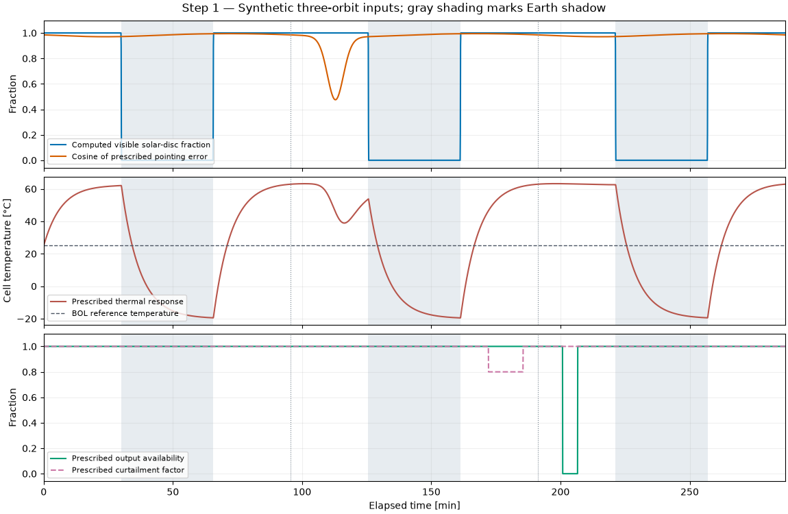
Circular period: 95.65 min; samples: 3,601; cadence: 4.78 s
reference_power_w is the ideal output counterfactual: the BOL array
reference with unity transfer. All final powers use the same converter-output
boundary. The synthetic actual signal is perturbed deliberately; no physical
cause is attached to that residual by the accounting API.
reference = opv.PvwattsReference(
    pdc0_w=1_000.0,
    gamma_pdc_per_c=-0.003,
    reference_irradiance_w_m2=1361.0,
    reference_temperature_c=25.0,
)
frame = opv.pvwatts_loss_chain(
    reference,
    am0_irradiance_w_m2=am0_irradiance,
    illumination_fraction=illumination,
    cosine_aoi=cosine_aoi,
    spectral_factor=1.01,
    optical_factor=0.98,
    cell_temperature_c=temperature_c,
    degradation_factor=0.94,
    mismatch_factor=0.985,
    wiring_efficiency=0.99,
    conversion_efficiency=0.95,
    power_limit_w=780.0,
    availability_factor=availability,
    curtailment_factor=curtailment,
)
frame["timestamp"] = pd.Timestamp("2026-01-01T00:00:00Z") + pd.to_timedelta(time_s, unit="s")
frame["expected_power_w"] = frame["reference_power_w"]
synthetic_residual_fraction = 0.008 * np.sin(2 * np.pi * orbit_phase / 0.09) - 0.075 * np.exp(
    -0.5 * ((orbit_phase - 2.82) / 0.055) ** 2
)
frame["actual_power_w"] = frame["modeled_power_w"] * (1.0 + synthetic_residual_fraction)

stages = [
    opv.LossStage(
        "distance",
        "after_irradiance_w",
        "solar_resource",
        "Prescribed Sun vector; inverse-square AM0",
    ),
    opv.LossStage(
        "eclipse", "after_eclipse_w", "geometry", "Computed finite solar-disc occultation"
    ),
    opv.LossStage(
        "pointing", "after_pointing_w", "geometry", "Prescribed Sun-pointing error and maneuver"
    ),
    opv.LossStage(
        "spectral", "after_spectral_w", "optical", "Assumed 1.01 relative spectral correction"
    ),
    opv.LossStage(
        "optical",
        "after_optical_w",
        "optical",
        "Assumed 0.98 incremental transmission relative to BOL",
    ),
    opv.LossStage(
        "temperature",
        "after_temperature_w",
        "temperature",
        "Toy thermal history; assumed -0.003/C coefficient",
    ),
    opv.LossStage(
        "degradation",
        "after_degradation_w",
        "degradation",
        "Assumed fixed 0.94 lifetime factor; no dose inference",
    ),
    opv.LossStage("mismatch", "after_mismatch_w", "electrical", "Assumed 0.985 mismatch factor"),
    opv.LossStage("wiring", "after_wiring_w", "electrical", "Assumed 0.99 wiring efficiency"),
    opv.LossStage(
        "conversion", "after_conversion_w", "conversion", "Assumed 0.95 DC/DC efficiency"
    ),
    opv.LossStage(
        "clipping", "after_clipping_w", "operations", "Prescribed 780 W cap on converter output"
    ),
    opv.LossStage(
        "availability", "after_availability_w", "operations", "Prescribed output disable event"
    ),
    opv.LossStage(
        "curtailment",
        "modeled_power_w",
        "operations",
        "Prescribed 0.8 output multiplier during command",
    ),
]
breakdown = opv.power_loss_breakdown(frame, stages)
summary = opv.summarize_power_losses(breakdown, max_gap_s=1.1 * step_s)

fig, axes = plt.subplots(2, 1, figsize=(11.5, 7.0), sharex=True, layout="constrained")
axes[0].plot(
    time_min,
    frame["expected_power_w"],
    color="#6B7280",
    linestyle="--",
    label="Ideal output reference (unity transfer)",
)
axes[0].plot(
    time_min,
    frame["after_wiring_w"],
    color="#56B4E9",
    linewidth=1,
    label="Array-side DC after wiring",
)
axes[0].plot(
    time_min,
    frame["modeled_power_w"],
    color="#0072B2",
    linewidth=1.8,
    label="Modeled converter output",
)
axes[0].plot(
    time_min,
    frame["actual_power_w"],
    color="#CC79A7",
    linewidth=1,
    label="SYNTHETIC actual at converter output",
)
axes[0].set(ylabel="Power [W]", ylim=(-30, 1_100))
axes[0].legend(loc="upper center", ncols=2, fontsize=8)
residual_w = breakdown.samples["unexplained_loss_w"].to_numpy()
axes[1].plot(time_min, residual_w, color="#4B5563", linewidth=1)
axes[1].fill_between(
    time_min,
    0,
    residual_w,
    where=residual_w >= 0,
    color="#D55E00",
    alpha=0.5,
    label="Model above SYNTHETIC actual",
)
axes[1].fill_between(
    time_min,
    0,
    residual_w,
    where=residual_w < 0,
    color="#009E73",
    alpha=0.5,
    label="SYNTHETIC actual above model",
)
axes[1].axhline(0, color="#4B5563", linewidth=0.7)
axes[1].set(ylabel="Unexplained residual [W]", xlabel="Elapsed time [min]")
axes[1].legend(loc="upper left", fontsize=8)
for ax in axes:
    shade_eclipses(ax)
fig.suptitle("Step 2 — Model and SYNTHETIC actual; a residual is not a fault diagnosis")
plt.show()
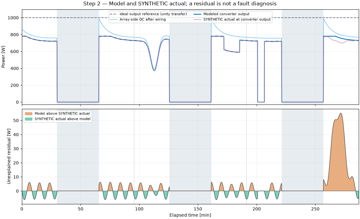
Contributions are integrated on common valid intervals. Positive loss subtracts energy; negative loss adds a gain. The gray residual is kept apart from the scenario’s explicitly supplied physical and operational stages.
totals = summary.totals.iloc[0]
component_names = [stage.name for stage in stages] + ["unexplained"]
components = summary.components.set_index("component").loc[component_names]
losses_wh = components["net_loss_wh"].to_numpy()
labels = (
    ["Ideal\nreference"] + [name.capitalize() for name in component_names] + ["SYNTHETIC\nactual"]
)
fig, ax = plt.subplots(figsize=(13.5, 5.8), layout="constrained")
remaining_wh = float(totals["expected_energy_wh"])
ax.bar(0, remaining_wh, color="#0072B2", width=0.7)
ax.text(0, remaining_wh + 65, f"{remaining_wh:,.0f}", ha="center", fontsize=8)
for position, (name, loss_wh) in enumerate(zip(component_names, losses_wh, strict=True), start=1):
    next_wh = remaining_wh - loss_wh
    color = "#6B7280" if name == "unexplained" else ("#D55E00" if loss_wh >= 0 else "#009E73")
    ax.plot(
        [position - 0.65, position - 0.35],
        [remaining_wh, remaining_wh],
        color="#73808C",
        linewidth=0.8,
    )
    ax.bar(position, abs(loss_wh), bottom=min(remaining_wh, next_wh), color=color, width=0.7)
    ax.text(position, max(remaining_wh, next_wh) + 65, f"{-loss_wh:+.0f}", ha="center", fontsize=8)
    remaining_wh = next_wh
last = len(labels) - 1
actual_wh = float(totals["actual_energy_wh"])
ax.plot([last - 0.65, last - 0.35], [remaining_wh, remaining_wh], color="#73808C", linewidth=0.8)
ax.bar(last, actual_wh, color="#0072B2", width=0.7)
ax.text(last, actual_wh + 65, f"{actual_wh:,.0f}", ha="center", fontsize=8)
ax.set(
    xticks=range(len(labels)),
    xticklabels=labels,
    ylabel="Energy over three orbits [Wh]",
    title="Step 3 — Ideal reference - ordered losses + gains = SYNTHETIC actual",
    ylim=(0, float(totals["expected_energy_wh"]) * 1.12),
)
ax.tick_params(axis="x", labelrotation=50, labelsize=8)
ax.legend(
    handles=[
        Patch(color="#D55E00", label="Prescribed/computed loss"),
        Patch(color="#009E73", label="Gain"),
        Patch(color="#6B7280", label="Unexplained residual"),
    ],
    loc="upper right",
    fontsize=8,
)
ax.grid(axis="y", alpha=0.2)
plt.show()
print("Three-orbit energy balance [Wh]:")
print(
    summary.totals[
        [
            "expected_energy_wh",
            "modeled_energy_wh",
            "actual_energy_wh",
            "attributed_energy_wh",
            "unexplained_energy_wh",
            "coverage_fraction",
        ]
    ]
    .round(3)
    .to_string(index=False)
)
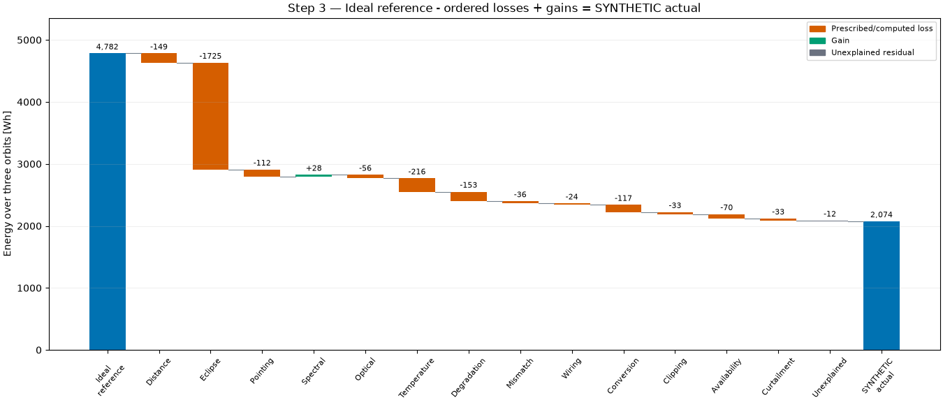
Three-orbit energy balance [Wh]:
 expected_energy_wh  modeled_energy_wh  actual_energy_wh  attributed_energy_wh  unexplained_energy_wh  coverage_fraction
           4782.494           2085.913          2073.986              2696.581                 11.928                1.0
Each orbit includes both endpoint samples, so its trapezoidal integral covers exactly one complete revolution. Repeated boundary timestamps occur only in different groups. No interval is integrated across orbit groups. Gross losses and gains are shown separately; their signed difference is the net category contribution. Their positive totals need not equal the total positive expected-minus-actual gap, because different components can cancel. Opposing stages within a category are combined before that category’s loss and gain intervals are integrated: the spectral gain offsets part of the optical loss in their shared category.
orbit_frames = []
for orbit in range(3):
    start = orbit * samples_per_orbit
    stop = (orbit + 1) * samples_per_orbit
    part = frame.iloc[start : stop + 1].copy()
    part["orbit"] = orbit + 1
    orbit_frames.append(part)
grouped = opv.power_loss_breakdown(
    pd.concat(orbit_frames, ignore_index=True), stages, group_columns=("orbit",)
)
orbit_summary = opv.summarize_power_losses(grouped, max_gap_s=1.1 * step_s)
category_labels = {
    "solar_resource": "Solar distance",
    "geometry": "Eclipse + pointing",
    "optical": "Spectrum + optical",
    "temperature": "Temperature",
    "degradation": "Assumed degradation",
    "electrical": "Mismatch + wiring",
    "conversion": "Conversion",
    "operations": "Output cap + commands",
    "unexplained": "Unexplained",
}
categories = summary.categories.set_index("category").loc[list(category_labels)]
fig, axes = plt.subplots(
    1, 2, figsize=(13, 5.8), layout="constrained", gridspec_kw={"width_ratios": [1.0, 1.45]}
)
x = np.arange(3)
for offset, column, color, label in (
    (-0.25, "expected_energy_wh", "#9CA3AF", "Ideal output reference"),
    (0.0, "modeled_energy_wh", "#0072B2", "Modeled output"),
    (0.25, "actual_energy_wh", "#CC79A7", "SYNTHETIC actual"),
):
    bars = axes[0].bar(
        x + offset, orbit_summary.totals[column], width=0.24, color=color, label=label
    )
    axes[0].bar_label(bars, fmt="%.0f", fontsize=8, padding=3)
axes[0].set(
    xticks=x,
    xticklabels=["Orbit 1", "Orbit 2", "Orbit 3"],
    ylabel="Energy [Wh]",
    title="Complete-orbit energy, same comparison boundary",
)
axes[0].legend(loc="upper right", fontsize=8)
axes[0].set_ylim(0, orbit_summary.totals["expected_energy_wh"].max() * 1.35)
axes[0].grid(axis="y", alpha=0.2)
y = np.arange(len(categories))
loss_bars = axes[1].barh(
    y - 0.16, categories["loss_wh"], height=0.3, color="#D55E00", label="Gross loss"
)
gain_bars = axes[1].barh(
    y + 0.16,
    -categories["gain_wh"],
    height=0.3,
    color="#009E73",
    label="Gross gain (drawn negative)",
)
axes[1].bar_label(loss_bars, fmt="%.1f", fontsize=8, padding=3)
axes[1].bar_label(
    gain_bars,
    labels=[f"{-value:.1f}" if value >= 0.05 else "" for value in categories["gain_wh"]],
    fontsize=8,
    padding=3,
)
axes[1].axvline(0, color="#4B5563", linewidth=0.7)
axes[1].set(
    yticks=y,
    yticklabels=list(category_labels.values()),
    xlabel="Three-orbit energy contribution [Wh]",
    title="Category totals keep losses and gains separate",
)
axes[1].invert_yaxis()
axes[1].margins(x=0.18)
axes[1].legend(loc="lower right", fontsize=8)
axes[1].grid(axis="x", alpha=0.2)
fig.suptitle("Step 4 — Grouped energy accounting for a SYNTHETIC scenario")
plt.show()
print("Per-orbit support and energy [Wh]:")
print(
    orbit_summary.totals[
        [
            "orbit",
            "expected_energy_wh",
            "modeled_energy_wh",
            "actual_energy_wh",
            "coverage_fraction",
        ]
    ]
    .round(3)
    .to_string(index=False)
)
print("Evidence remains explicit:")
print(summary.components[["component", "category", "evidence"]].to_string(index=False))
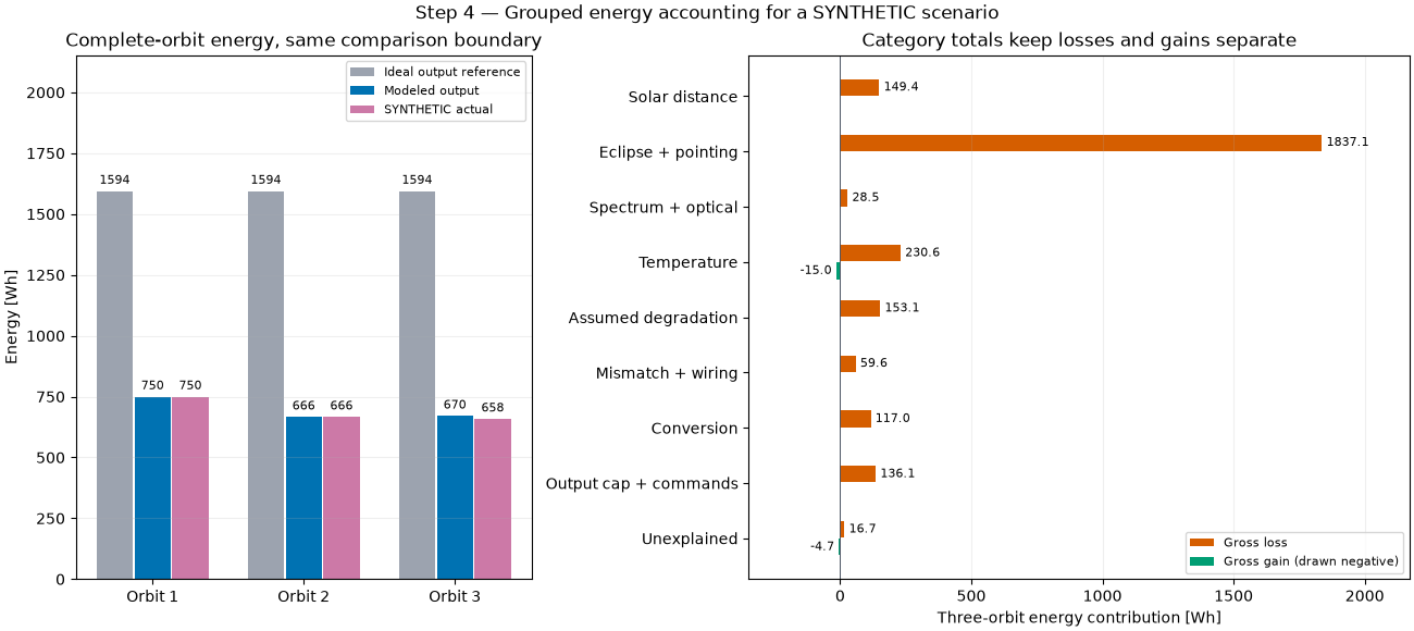
Per-orbit support and energy [Wh]:
 orbit  expected_energy_wh  modeled_energy_wh  actual_energy_wh  coverage_fraction
     1            1594.165            749.523           749.592                1.0
     2            1594.165            666.257           666.355                1.0
     3            1594.165            670.133           658.039                1.0
Evidence remains explicit:
   component       category                                                     evidence
    distance solar_resource                    Prescribed Sun vector; inverse-square AM0
     eclipse       geometry                       Computed finite solar-disc occultation
    pointing       geometry                   Prescribed Sun-pointing error and maneuver
    spectral        optical                    Assumed 1.01 relative spectral correction
     optical        optical        Assumed 0.98 incremental transmission relative to BOL
 temperature    temperature            Toy thermal history; assumed -0.003/C coefficient
 degradation    degradation        Assumed fixed 0.94 lifetime factor; no dose inference
    mismatch     electrical                                Assumed 0.985 mismatch factor
      wiring     electrical                               Assumed 0.99 wiring efficiency
  conversion     conversion                                Assumed 0.95 DC/DC efficiency
    clipping     operations                     Prescribed 780 W cap on converter output
availability     operations                              Prescribed output disable event
 curtailment     operations              Prescribed 0.8 output multiplier during command
 unexplained    unexplained Final modeled power minus actual power; cause not identified
Eclipse is a large, expected geometric reduction from the ideal reference. Pointing and output commands distinguish the three otherwise similar orbits. The spectral correction and cold-cell periods demonstrate genuine signed gains within the prescribed model. Reordering stages changes their assigned incremental contributions, and a different baseline changes what counts as loss. A real mission analysis needs calibrated reference data, matched timestamps and electrical boundaries, and independent evidence for each attribution. Actual-minus-model alone cannot establish degradation or faults.
Total running time of the script: (0 minutes 1.096 seconds)