Note
Go to the end to download the full example code.
BUPT-1 measured electrical energy budget#
This offline view displays precomputed aggregate measurements, generated
by analysis/bupt1_energy_budget/run.py from the pinned public BUPT-1
archive. Raw telemetry is not bundled because its repository has not declared
a redistribution licence. The analysis can download and reproduce the numbers.
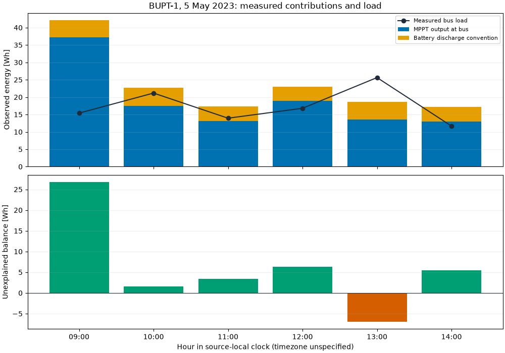
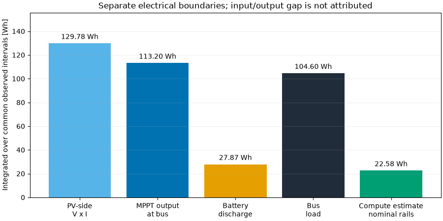
The source-local six-hour window contains native measurements during active computing. Its timezone is unspecified; no UTC or eclipse alignment is claimed. Input PV power, MPPT output and spacecraft bus load remain separate boundaries.
import json
from pathlib import Path

import matplotlib.pyplot as plt
import numpy as np

import orbitalpv as opv
directory = Path(__file__).resolve().parent if "__file__" in globals() else Path.cwd()
path = directory / "_data/bupt1_energy_budget_aggregate.json"
summary = json.loads(path.read_text())
print("Public connector:", opv.SatelliteCOTSConnector.__name__)
print("Source commit:", summary["source_commit"])
print("Source SHA-256:", summary["source_sha256"])
print("Clock interpretation:", summary["timestamp_basis"])
print("Measured rows:", summary["source_rows"])
print("Precomputed observed-time budget:", summary["bus_energy_budget"])
print(
    "Compute branch estimate from measured currents and nominal rails:",
    summary["compute_load_estimate"],
)
Public connector: SatelliteCOTSConnector
Source commit: 951b41521351d535b7c2354916d9c4991602e8c7
Source SHA-256: 5d761d0bb65730cdbdb364f9c8706e9469bbbc6049cc0ed0b22d95ead8d656fa
Clock interpretation: Source-local clock; timezone unspecified
Measured rows: 21598
Precomputed observed-time budget: {'observed_duration_h': 5.999722222222222, 'timestamp_span_h': 5.999722222222222, 'coverage_fraction': 1.0, 'accepted_intervals': 21597, 'excluded_intervals': 0, 'max_gap_s': 2.0, 'solar_wh': 113.20013909444444, 'load_wh': 104.59703797986111, 'battery_discharge_wh': 27.87065722222222, 'unexplained_balance_wh': 36.47375833680556, 'battery_mode': 'discharge = -1 x source', 'interpretation': 'Observed-time energy; no missing periods filled or physical causes inferred'}
Compute branch estimate from measured currents and nominal rails: {'observed_energy_wh': 22.58029722222222, 'nonzero_compute_current_rows': 7349, 'atlas_nominal_rail_v': 12.1, 'raspberry_pi_nominal_rail_v': 5.1, 'boundary': 'Measured branch currents times source-code nominal rail voltages; estimated, not independently measured power'}
Battery sign follows the authors’ convention: negative source current is plotted as discharge. The disagreement stays unexplained. It cannot be assigned to converter loss, cell degradation or thermal effects from this dataset alone.
hourly = summary["hourly_observed_energy"]
x = np.arange(len(hourly))
solar = np.array([row["solar_wh"] for row in hourly])
battery = np.array([row["battery_discharge_wh"] for row in hourly])
load = np.array([row["load_wh"] for row in hourly])
residual = np.array([row["unexplained_balance_wh"] for row in hourly])
fig, axes = plt.subplots(2, 1, figsize=(10, 7), sharex=True, layout="constrained")
axes[0].bar(x, solar, color="#0072B2", label="MPPT output at bus")
axes[0].bar(x, battery, bottom=solar, color="#E69F00", label="Battery discharge convention")
axes[0].plot(x, load, "o-", color="#202C39", label="Measured bus load")
axes[0].set(
    ylabel="Observed energy [Wh]", title="BUPT-1, 5 May 2023: measured contributions and load"
)
axes[0].legend(loc="upper right", fontsize=8)
axes[1].bar(x, residual, color=np.where(residual >= 0, "#009E73", "#D55E00"))
axes[1].axhline(0, color="#202C39", linewidth=0.8)
axes[1].set(
    ylabel="Unexplained balance [Wh]",
    xlabel="Hour in source-local clock (timezone unspecified)",
    xticks=x,
    xticklabels=[row["hour"][11:16] for row in hourly],
)
for ax in axes:
    ax.grid(axis="y", alpha=0.2)
plt.show()
budget = summary["bus_energy_budget"]
input_budget = summary["input_output_comparison"]
fig, ax = plt.subplots(figsize=(9, 4.5), layout="constrained")
labels = [
    "PV-side\nV x I",
    "MPPT output\nat bus",
    "Battery\ndischarge",
    "Bus\nload",
    "Compute estimate\nnominal rails",
]
values = [
    input_budget["solar_wh"],
    budget["solar_wh"],
    budget["battery_discharge_wh"],
    budget["load_wh"],
    summary["compute_load_estimate"]["observed_energy_wh"],
]
bars = ax.bar(labels, values, color=["#56B4E9", "#0072B2", "#E69F00", "#202C39", "#009E73"])
ax.bar_label(bars, fmt="%.2f Wh", padding=4)
ax.set(
    ylabel="Integrated over common observed intervals [Wh]",
    ylim=(0, max(values) * 1.2),
    title="Separate electrical boundaries; input/output gap is not attributed",
)
ax.grid(axis="y", alpha=0.2)
plt.show()
Total running time of the script: (0 minutes 0.325 seconds)