Note
Go to the end to download the full example code.
Data-center wind procurement: annual energy versus hourly coverage#
News trigger (11 November 2026): BloombergNEF projects 2,354 TWh/year of worldwide data-center electricity demand in 2035, roughly 7% of global consumption, and separately tracks 181 GW of announced gas proposals near data centers. Those figures are BNEF forecasts/pipeline counts, not observations or committed installations.
Business decision: How many GW of wind nameplate capacity might an annual-energy PPA require at assumed capacity factors? Why does a nominal annual-MWh match not guarantee the hourly supply needed by data centers?
Primary source: BloombergNEF press release, 11 November 2026. The source is an attributed published forecast, not a licensed time series.
All wind CF, transmission-loss, hourly shape, storage and PPA shares below are ILLUSTRATIVE ASSUMPTIONS, not measured project values, model forecasts, or confidence intervals. The 168-hour matching demonstration is SYNTHETIC. See study guide.
1. Annual energy sensitivity against the reported demand forecast.#
import math

import matplotlib.pyplot as plt

from energy_methods.data_center_wind import screen_annual_wind, screen_hourly_wind

BNEF_FORECAST_TWH_2035 = 2354.0  # Forecast, not measured data.
BNEF_ANNOUNCED_GAS_GW = 181.0  # Pipeline, not forecast operating capacity.
assumed_delivery_loss = 0.06
capacity_factors = [0.30, 0.36, 0.42, 0.48, 0.54]
procurement_shares = [0.25, 0.50, 1.0]

fig, ax = plt.subplots(figsize=(9, 4.5), layout="constrained")
for fraction in procurement_shares:
    wind_gw = [
        screen_annual_wind(
            BNEF_FORECAST_TWH_2035, fraction, cf, assumed_delivery_loss
        ).required_wind_gw
        for cf in capacity_factors
    ]
    ax.plot(
        [100 * cf for cf in capacity_factors],
        wind_gw,
        marker="o",
        label=f"Annual procurement target {fraction:.0%}",
    )
    if fraction == 0.25:
        print(f"Illustrative 25% PPA at 42% wind CF: {wind_gw[2]:.1f} GW wind")
ax.set(
    xlabel="Assumed delivered-energy wind capacity factor before 6% loss (%)",
    ylabel="New wind nameplate for annual MWh matching (GW)",
    title="BNEF 2035 demand forecast: wind PPA *annual energy* screen",
)
ax.legend()
plt.show()
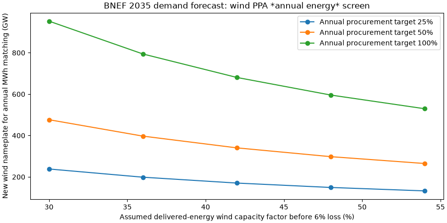
Illustrative 25% PPA at 42% wind CF: 170.2 GW wind
2. Explicitly synthetic weekly profile: zero-storage versus storage.#
A 100 MW CONSTANT site and 240 MW wind nameplate are entirely synthetic. Neither this week’s normalized wind nor the loading reflects a real location.
HOURS = 168
wind_cf_week = [
    min(
        0.82,
        max(
            0.03,
            0.42 + 0.20 * math.sin(2 * math.pi * h / 70) + 0.12 * math.sin(2 * math.pi * h / 19),
        ),
    )
    for h in range(HOURS)
]
site_mw = [100.0] * HOURS
bess_hours = [0, 1, 2, 4, 8, 12]
illustrative_wind_mw = 240.0
results = [
    screen_hourly_wind(
        wind_cf_week,
        site_mw,
        wind_capacity_mw=illustrative_wind_mw,
        delivery_loss_fraction=assumed_delivery_loss,
        battery_power_mw=100.0,
        battery_energy_mwh=100.0 * hours,
        battery_round_trip_efficiency=0.9,
    )
    for hours in bess_hours
]
energy_match = 100 * results[0].energy_matched_fraction
hourly_coverage = [100 * r.hourly_served_fraction for r in results]
print(f"SYNTHETIC weekly aggregate energy match: {energy_match:.1f}%")
print(f"SYNTHETIC no-storage hourly supplied share: {hourly_coverage[0]:.1f}%")
print(f"SYNTHETIC 12h storage hourly supplied share: {hourly_coverage[-1]:.1f}%")

fig, ax = plt.subplots(figsize=(9, 4.5), layout="constrained")
ax.plot(bess_hours, hourly_coverage, marker="o", label="Hourly wind/BESS served (%)")
ax.axhline(
    energy_match,
    linestyle="--",
    color="black",
    label="Window-total energy match ceiling (%)",
)
ax.set(
    xlabel="Assumed battery duration at 100 MW (hours)",
    ylabel="Illustrative share of demand (%)",
    ylim=(0, 105),
    title="SYNTHETIC 168h: annual-style energy accounting != hourly supply",
)
ax.legend()
plt.show()
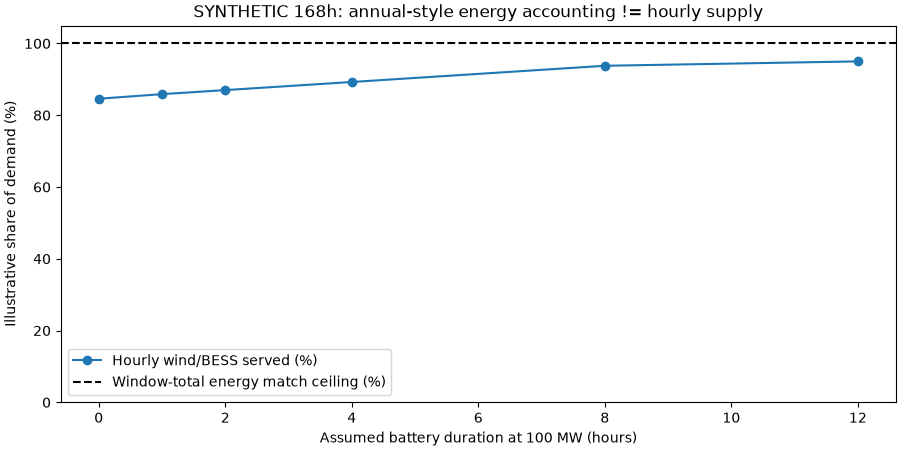
SYNTHETIC weekly aggregate energy match: 100.0%
SYNTHETIC no-storage hourly supplied share: 84.6%
SYNTHETIC 12h storage hourly supplied share: 95.0%
3. Technical interpretation.#
The gas pipeline number 181 GW is NOT compared one-to-one to wind capacity: dispatchable MW and intermittent nameplate GW are not interchangeable. BESS is initially empty and can only charge from otherwise-surplus wind. Energy matching is a generous aggregate-energy bookkeeping ceiling; it does not establish contractual certificates, deliverability or 24/7 CFE. No capex, costs, weather years, 2035 hourly forecast, grid connection, congestion, emissions, demand response or operational reliability is modeled. Offline: uv run –no-sync python examples/analysis/plot_bnef_data_center_wind_2026.py
Total running time of the script: (0 minutes 0.162 seconds)