Note
Go to the end to download the full example code.
Spain system-adjustment costs and battery revenue-screening boundaries#
Red Eléctrica reported a 26.4% year-on-year increase in energy used for technical restrictions and a 43.4% increase in their cost to demand for January-October 2026 (press note 3 November 2026). The reported figures are system aggregates, not battery revenues.
Business question: Which part of the apparent cost increase reflects energy volume, and what flat price differential would cover round-trip losses and a hypothetical variable battery-wear allowance?
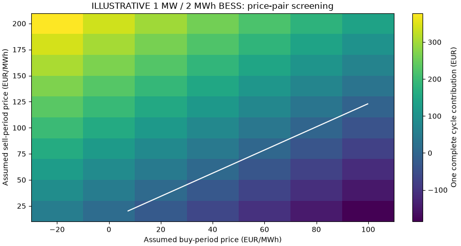
The first plot uses official reported aggregate changes. The second uses ILLUSTRATIVE price scenarios, not measured Spanish intraday prices. The reported 214.73 EUR/MWh technical-restriction remuneration and 82.10 EUR/MWh day-ahead mean are not comparable tradable legs and are never passed to the battery model. This case cannot forecast storage or ancillary-service returns.
Reproduction and limitations: docs/ree-adjustment-bess.md.
import json
from pathlib import Path

import matplotlib.pyplot as plt
import numpy as np

from energy_methods.grid_adjustment_bess import (
    infer_aggregate_unit_cost_growth,
    screen_complete_bess_cycle,
)
Published aggregate growth, not an observed hourly timeseries. Sphinx-Gallery executes examples without setting __file__. Discover the source-tree fixture from the invocation path or any ancestor, offline.
script_path = Path(globals().get("__file__", Path.cwd() / "plot_ree_adjustment_bess.py")).resolve()
source_file = next(
    (
        candidate
        for ancestor in (script_path.parent, *script_path.parents)
        for candidate in (
            ancestor / "ree_adjustment_20261103.json",
            ancestor / "examples/analysis/ree_adjustment_20261103.json",
        )
        if candidate.is_file()
    ),
    None,
)
if source_file is None:
    raise FileNotFoundError("Missing attributed REE adjustment source snapshot")
snapshot = json.loads(source_file.read_text(encoding="utf-8"))
reported = snapshot["reported"]
growth = infer_aggregate_unit_cost_growth(
    reported["technical_restrictions_energy_yoy_pct"],
    reported["technical_restrictions_cost_to_demand_yoy_pct"],
)
print("EVIDENCE:", snapshot["evidence_class"], snapshot["source"]["url"])
print(f"REE reported volume index: {growth.energy_index:.3f} (2025 period = 1)")
print(f"REE reported cost index: {growth.cost_index:.3f} (2025 period = 1)")
print(f"Implied aggregate cost/MWh change: {growth.implied_unit_cost_growth_pct:+.2f}%")
print("Not a price spread or an estimate of merchant/BESS earnings.")

fig, ax = plt.subplots(figsize=(8.5, 4), layout="constrained")
ax.bar(
    ["2025 cost index", "2026 volume effect", "2026 reported cost"],
    [100.0, 100 * growth.energy_index, 100 * growth.cost_index],
)
ax.set(
    ylabel="Index (previous corresponding period = 100)",
    title="REE technical restrictions: reported volume vs cost growth",
)
ax.text(1, 100 * growth.energy_index + 1, "+26.4% volume", ha="center")
ax.text(2, 100 * growth.cost_index + 1, "+43.4% total cost", ha="center")
ax.set_ylim(0, 165)
plt.show()
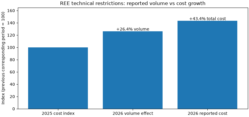
EVIDENCE: official_reported_aggregate_not_asset_measurement https://www.ree.es/es/actualidad/nota-de-prensa/2026/11/servicios-ajuste-elevan-4350-millones-euros-ingresos-generadoras-octubre
REE reported volume index: 1.264 (2025 period = 1)
REE reported cost index: 1.434 (2025 period = 1)
Implied aggregate cost/MWh change: +13.45%
Not a price spread or an estimate of merchant/BESS earnings.
Pure HYPOTHETICAL cycle economics: assumed 1 MW / 2 MWh battery, two separate 2-hour charging/discharging windows, 90% round-trip efficiency and 12 EUR/MWh delivered allowance for incremental wear. Each grid cell commits the physically feasible one-cycle energy volume. NOT a market price history, dispatch optimizer or projected net project profit.
buy_prices = np.arange(-20, 101, 20, dtype=float)
sell_prices = np.arange(20, 201, 20, dtype=float)
margin = np.zeros((len(sell_prices), len(buy_prices)))
for i, sell in enumerate(sell_prices):
    for j, buy in enumerate(buy_prices):
        result = screen_complete_bess_cycle(
            charge_price_eur_mwh=float(buy),
            sale_price_eur_mwh=float(sell),
            battery_power_mw=1.0,
            usable_energy_mwh=2.0,
            charging_hours=2.0,
            discharging_hours=2.0,
            round_trip_efficiency=0.9,
            wear_eur_per_delivered_mwh=12.0,
        )
        margin[i, j] = result.contribution_eur

fig, ax = plt.subplots(figsize=(9, 4.8), layout="constrained")
image = ax.imshow(
    margin,
    origin="lower",
    aspect="auto",
    extent=[
        buy_prices[0] - 10,
        buy_prices[-1] + 10,
        sell_prices[0] - 10,
        sell_prices[-1] + 10,
    ],
)
fig.colorbar(image, ax=ax, label="One complete cycle contribution (EUR)")
ax.contour(buy_prices, sell_prices, margin, levels=[0], colors="white", linewidths=1.5)
ax.set(
    title="ILLUSTRATIVE 1 MW / 2 MWh BESS: price-pair screening",
    xlabel="Assumed buy-period price (EUR/MWh)",
    ylabel="Assumed sell-period price (EUR/MWh)",
)
plt.show()
base = screen_complete_bess_cycle(
    charge_price_eur_mwh=60,
    sale_price_eur_mwh=120,
    battery_power_mw=0,
    usable_energy_mwh=0,
    charging_hours=2,
    discharging_hours=2,
)
example = screen_complete_bess_cycle(
    charge_price_eur_mwh=60,
    sale_price_eur_mwh=120,
    battery_power_mw=1,
    usable_energy_mwh=2,
    charging_hours=2,
    discharging_hours=2,
    round_trip_efficiency=0.9,
    wear_eur_per_delivered_mwh=12,
)
print(f"HYPOTHETICAL no-storage contribution: {base.contribution_eur:.2f} EUR")
print(f"HYPOTHETICAL cycle purchased: {example.charged_mwh:.2f} MWh")
print(f"HYPOTHETICAL cycle delivered: {example.delivered_mwh:.2f} MWh")
print(f"HYPOTHETICAL one-cycle margin: {example.contribution_eur:.2f} EUR")
print(f"Break-even sell price: {example.break_even_sale_price_eur_mwh:.2f} EUR/MWh")
print("This is not revenue from technical restrictions or a financeable BESS forecast.")
HYPOTHETICAL no-storage contribution: 0.00 EUR
HYPOTHETICAL cycle purchased: 2.00 MWh
HYPOTHETICAL cycle delivered: 1.80 MWh
HYPOTHETICAL one-cycle margin: 74.40 EUR
Break-even sell price: 78.67 EUR/MWh
This is not revenue from technical restrictions or a financeable BESS forecast.
Total running time of the script: (0 minutes 0.196 seconds)