Note
Go to the end to download the full example code.
Hams Hall battery: audit 3.5-hour household-equivalent delivery#
On 2 November 2026, developer BW ESS announced Hams Hall phase one commercial operations at 350 MW / 1,243 MWh. The proposed second phase would bring totals to 400 MW / 1,424 MWh. BW ESS describes the completed project as capable of supporting about 1.3 million homes for up to 3.5 hours. These are developer-published nameplate and equivalence claims; not metered AC discharge, independently established usable energy or typical coincident household peak loads.
Primary developer project page: https://bw-ess.com/projects/hams-hall The full dated press-release URL is cited in docs/hams-hall-bess-service.md.
Business question: under what SOC, capacity retention and discharge-loss assumptions can the stated energy and power envelope support 1.3 million hypothetical constant-average-demand households for 3.5 hours?
Scenario parameters below are ASSUMED; all measured site duty cycles, household load profiles and actual AC energy basis are UNKNOWN. The result is an engineering bound, not grid connection, reserve certification or revenue.
import matplotlib.pyplot as plt

from energy_methods.bess_service_envelope import maximum_households, screen_bess_service

first_phase = (350.0, 1243.0)  # Developer-reported MW / MWh, 2 Nov 2026
full_build = (400.0, 1424.0)  # Developer-reported FUTURE total MW / MWh
claimed_homes = 1_300_000  # Developer's approximate marketing equivalence
claimed_hours = 3.5
Baseline: ideal use of declared MWh without losses. If MWh already denotes AC-deliverable capacity, efficiency=1 is appropriate, otherwise a discharge conversion is needed. The public statement does not resolve the energy basis.
for phase, (power, energy) in (
    ("Operating first phase", first_phase),
    ("Proposed full build", full_build),
):
    ideal = screen_bess_service(power, energy, claimed_hours, target_power_mw=power)
    print(
        f"{phase}: nominal duration={energy / power:.3f} h; "
        f"3.5-hour ideal export ceiling={ideal.sustainable_power_mw:.1f} MW"
    )

# Claimed homes imply an average power ceiling of 400 MW / 1.3m = 0.308 kW/home.
# This is not an actual mean household use measurement or a peak-load claim.
print(
    "Claim-implied per-home power ceiling (full build): "
    f"{1000 * full_build[0] / claimed_homes:.3f} kW/home"
)
Operating first phase: nominal duration=3.551 h; 3.5-hour ideal export ceiling=350.0 MW
Proposed full build: nominal duration=3.560 h; 3.5-hour ideal export ceiling=400.0 MW
Claim-implied per-home power ceiling (full build): 0.308 kW/home
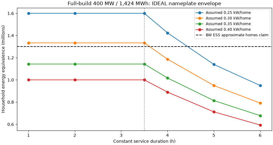
HYPOTHETICAL household-load sensitivity, with no operational reserve or loss.
hours = [1, 2, 3.5, 4, 5, 6]
loads_kw = (0.25, 0.30, 0.35, 0.40)
fig, ax = plt.subplots(figsize=(9, 4.8), layout="constrained")
for load in loads_kw:
    envelopes = [screen_bess_service(*full_build, h) for h in hours]
    ax.plot(
        hours,
        [maximum_households(e, load) / 1e6 for e in envelopes],
        marker="o",
        label=f"Assumed {load:.2f} kW/home",
    )
ax.axhline(
    claimed_homes / 1e6, color="black", linestyle="--", label="BW ESS approximate homes claim"
)
ax.axvline(claimed_hours, color="gray", linestyle=":")
ax.set(
    xlabel="Constant service duration (h)",
    ylabel="Household energy equivalence (millions)",
    title="Full-build 400 MW / 1,424 MWh: IDEAL nameplate envelope",
)
ax.legend(fontsize="small")
plt.show()
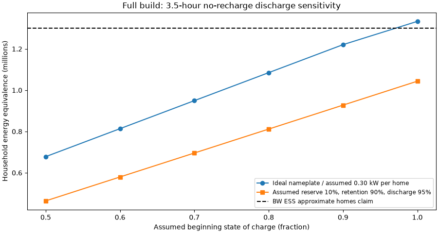
ASSUMED starting SOC and headroom stress test; 0.30 kW/home is illustrative.
initial_soc = [0.5, 0.6, 0.7, 0.8, 0.9, 1.0]
reserve_soc = 0.10
usable_fraction = 0.90  # assumed retained available capacity, NOT measured SOH
eta_discharge = 0.95  # assumed energy conversion, only if MWh declared upstream AC
stressed = [
    screen_bess_service(
        *full_build,
        claimed_hours,
        initial_soc_fraction=soc,
        reserve_soc_fraction=reserve_soc,
        usable_capacity_fraction=usable_fraction,
        discharge_efficiency=eta_discharge,
    )
    for soc in initial_soc
]
ideal = [
    screen_bess_service(
        *full_build,
        claimed_hours,
        initial_soc_fraction=soc,
        reserve_soc_fraction=0,
        usable_capacity_fraction=1,
        discharge_efficiency=1,
    )
    for soc in initial_soc
]
fig, ax = plt.subplots(figsize=(9, 4.8), layout="constrained")
ax.plot(
    initial_soc,
    [maximum_households(e, 0.30) / 1e6 for e in ideal],
    marker="o",
    label="Ideal nameplate / assumed 0.30 kW per home",
)
ax.plot(
    initial_soc,
    [maximum_households(e, 0.30) / 1e6 for e in stressed],
    marker="s",
    label="Assumed reserve 10%, retention 90%, discharge 95%",
)
ax.axhline(
    claimed_homes / 1e6, color="black", linestyle="--", label="BW ESS approximate homes claim"
)
ax.set(
    xlabel="Assumed beginning state of charge (fraction)",
    ylabel="Household energy equivalence (millions)",
    title="Full build: 3.5-hour no-recharge discharge sensitivity",
)
ax.legend(fontsize="small")
plt.show()
Reproduce: uv run –no-sync python examples/analysis/plot_hams_hall_bess_service.py Hypothetical constant mean power is NOT a sampled UK demand profile. This screen assumes no recharge, no dynamic dispatch, no batteries’ DC/AC capacity reconciliation, and no battery telemetry or external grid service commitments.
Total running time of the script: (0 minutes 0.177 seconds)