Note
Go to the end to download the full example code.
Canary Islands: nine PVDeg degradation-mechanism maps#
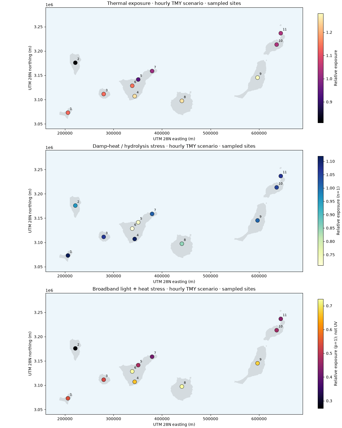
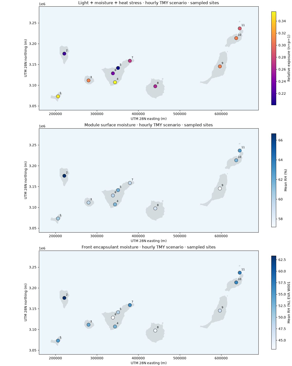
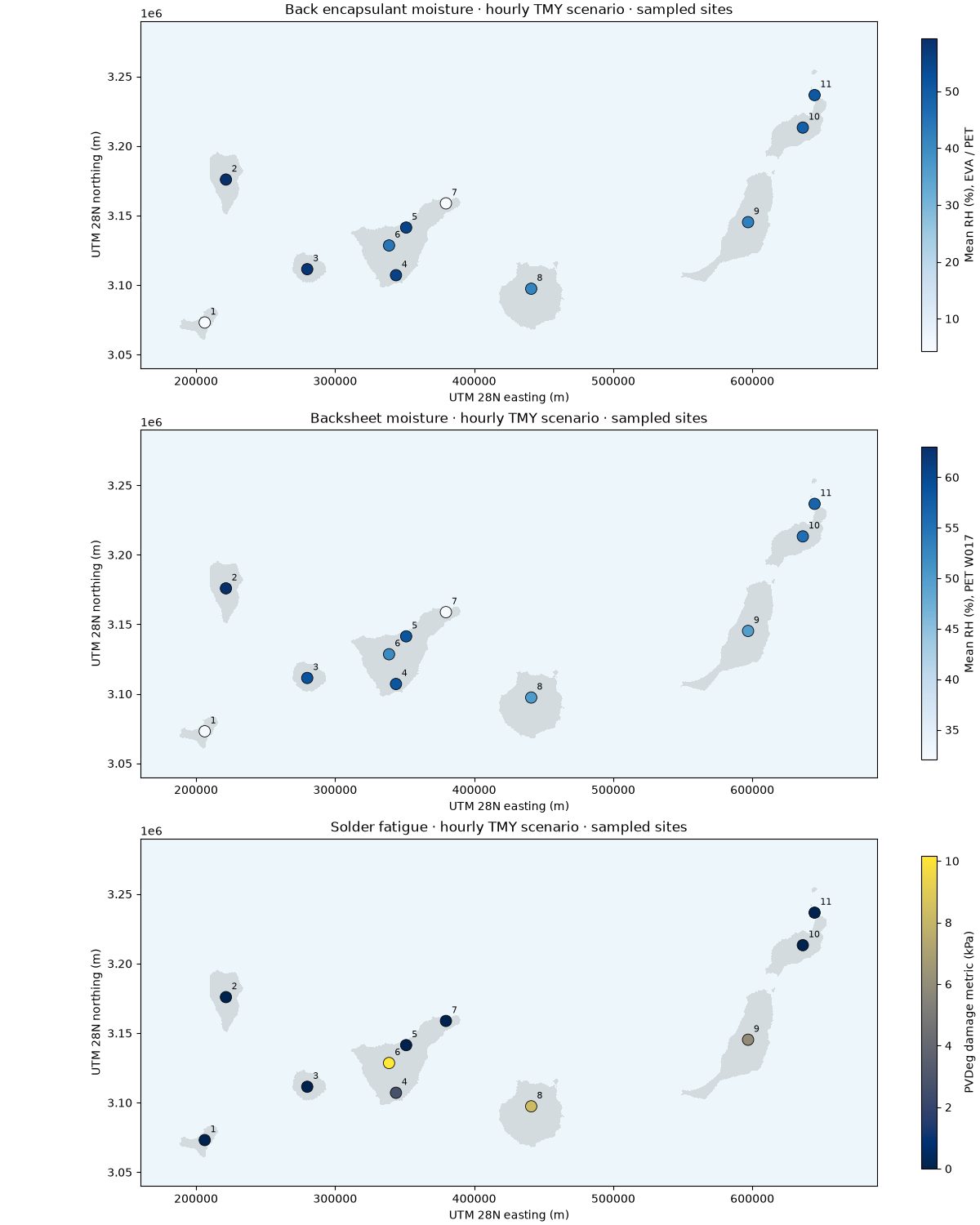
This complements the 100 m thermal map with hourly-weather mechanism screening at eleven locations across eight islands. PVGIS supplies modeled TMY irradiance, humidity, temperature and wind, selected from 2005-2023. Every result below is recomputed offline with PVDeg 0.7.4.
The maps cover thermal, damp-heat, broadband light-assisted and combined stress; module-surface, front/back encapsulant and backsheet moisture; and solder fatigue. They are scenario metrics, not annual power loss or remaining lifetime. Do not add the metrics together: they have different units and overlapping physics.
Markers show the actual sampling locations. The coastlines use the existing
100 m climate masks for context only. No humidity/irradiance downscaling or spatial
interpolation is performed. These are not 100 m degradation predictions.
See the guide for parameters, coverage,
missing mechanisms and reproducible input acquisition. Inputs and metadata are
available in the repository’s examples/analysis/pvdeg_canary_weather directory.
from pathlib import Path

import matplotlib.pyplot as plt
import numpy as np
import rasterio
from matplotlib.colors import ListedColormap
from rasterio.plot import plotting_extent
from rasterio.warp import transform

from energy_analysis.pvdeg_mechanisms import METRICS, analyze_manifest
Calculate every mechanism using hashed hourly inputs#
results = analyze_manifest(Path("pvdeg_canary_weather"))
print(results.round(3).to_string(index=False))
print("Weather: modeled PVGIS TMY; material / module parameters: scenarios")
print("No calibrated annual degradation rate, UV damage, PID or LeTID prediction")
x, y = transform("EPSG:4326", "EPSG:32628", results.longitude.tolist(), results.latitude.tolist())
          name  longitude  latitude  thermal  damp_heat  photothermal  combined  surface_rh  front_rh  back_rh  backsheet_rh  solder_fatigue
     El Hierro    -17.980    27.750    1.134      1.119         0.542     0.350      60.587    54.941    4.300        32.443           0.000
      La Palma    -17.850    28.680    0.810      0.956         0.268     0.216      66.665    63.356   59.331        62.998           0.000
     La Gomera    -17.240    28.110    1.135      1.062         0.529     0.309      59.796    53.784   58.132        58.964           0.000
Tenerife south    -16.590    28.080    1.253      1.108         0.663     0.356      61.477    52.771   55.514        58.496           2.684
Tenerife north    -16.520    28.390    0.938      0.731         0.475     0.201      61.773    49.282   55.405        58.589           0.000
         Teide    -16.644    28.272    1.142      0.710         0.728     0.237      60.013    43.053   44.214        52.114          10.169
         Anaga    -16.230    28.550    1.015      1.015         0.418     0.270      59.630    56.063    4.396        32.013           0.000
  Gran Canaria    -15.600    28.000    1.254      0.850         0.728     0.261      58.795    44.056   41.504        50.149           8.270
 Fuerteventura    -14.010    28.430    1.281      1.010         0.678     0.308      57.165    47.235   42.378        49.772           5.925
     Lanzarote    -13.600    29.040    1.035      1.047         0.468     0.307      61.563    56.653   49.192        55.377           0.000
   La Graciosa    -13.510    29.250    1.037      1.067         0.442     0.289      62.739    57.359   50.815        56.777           0.000
Weather: modeled PVGIS TMY; material / module parameters: scenarios
No calibrated annual degradation rate, UV damage, PID or LeTID prediction
Nine separate maps with their own units#
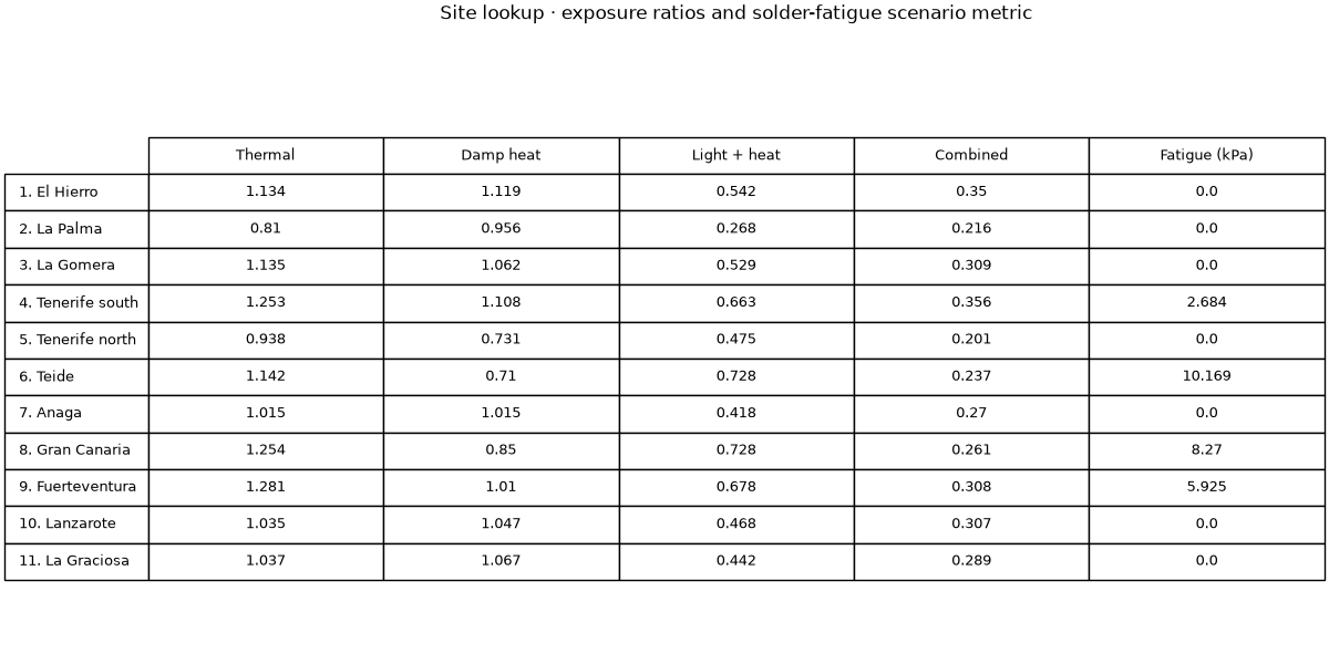
Numbered sites can be identified in the following table. Gray land is context, not a computed degradation surface. Color is only assigned to sampled points.
land = []
for path in sorted(Path(".").glob("pvdeg_canary_*.tif")):
    with rasterio.open(path) as dataset:
        mask = dataset.read(1, masked=True)
        land.append(
            (
                np.ma.array(np.ones(mask.shape), mask=mask.mask),
                plotting_extent(mask, dataset.transform),
            )
        )
for group in (list(METRICS)[:3], list(METRICS)[3:6], list(METRICS)[6:]):
    fig, axes = plt.subplots(3, 1, figsize=(12, 15), layout="constrained")
    for ax, key in zip(axes, group, strict=True):
        title, unit, cmap = METRICS[key]
        ax.set_facecolor("#edf6fb")
        for mask, extent in land:
            ax.imshow(
                mask, extent=extent, cmap=ListedColormap(["#d4dbdf"]), interpolation="nearest"
            )
        artist = ax.scatter(
            x, y, c=results[key], cmap=cmap, s=100, edgecolors="black", linewidths=0.6, zorder=3
        )
        for i, (east, north) in enumerate(zip(x, y, strict=True), start=1):
            ax.annotate(
                str(i),
                (east, north),
                xytext=(5, 7),
                textcoords="offset points",
                fontsize=8,
                zorder=4,
            )
        ax.set(
            xlim=(160000, 690000),
            ylim=(3040000, 3290000),
            title=f"{title} · hourly TMY scenario · sampled sites",
            xlabel="UTM 28N easting (m)",
            ylabel="UTM 28N northing (m)",
        )
        fig.colorbar(artist, ax=ax, label=unit, shrink=0.9)
Site comparison and interpretation#
The exposure ratios use 60 kJ/mol and a constant 25 C / 50% RH / 1000 W/m² reference. The light term uses broadband POA, not a UV spectrum. Moisture uses upstream EVA W001 / PET W017 defaults. Solder fatigue uses the upstream hourly calibration; it is not a percentage of failed joints or module power.
fig, ax = plt.subplots(figsize=(12, 6), layout="constrained")
ax.axis("off")
columns = ["thermal", "damp_heat", "photothermal", "combined", "solder_fatigue"]
labels = [f"{i}. {name}" for i, name in enumerate(results.name, start=1)]
table = ax.table(
    cellText=results[columns].round(3).to_numpy(),
    rowLabels=labels,
    colLabels=["Thermal", "Damp heat", "Light + heat", "Combined", "Fatigue (kPa)"],
    loc="center",
    cellLoc="center",
)
table.auto_set_font_size(False)
table.set_fontsize(9)
table.scale(1, 1.7)
ax.set_title("Site lookup · exposure ratios and solder-fatigue scenario metric", pad=25)
plt.show()
Total running time of the script: (0 minutes 3.428 seconds)