Note
Go to the end to download the full example code.
Dogger Bank C: offshore installation-vessel capacity and grid readiness#
Dated primary evidence: Dogger Bank Wind Farm, 4 November 2026, announced that Wind Apex is expected to join Seaway Ventus for Dogger Bank C in Q3 2027. Phase C has 87 turbines and 1.2 GW. These are public project announcements, NOT measured work rates, actual site conditions, or an operating forecast. Source: https://doggerbank.com/news/
Business question: How might a second installation vessel change the construction critical path and the opportunity for eventual renewable energy?
The daily planning method represents a common site-weather gate and per-vessel work-days-per-turbine, followed by a separate grid-ready gate. This exercise uses SYNTHETIC weather and ILLUSTRATIVE time, efficiency, capacity factor and price assumptions. It estimates neither the real Dogger Bank schedule nor an economic value agreed by the developer. Run entirely offline; no licensed generation data or API credentials are needed.
See source facts, formulas and scientific limits.
from __future__ import annotations

import random

import matplotlib.pyplot as plt
import numpy as np

from energy_methods.wind_installation import (
    commissioning_opportunity_mwh,
    simulate_installation,
)
1. Separate dated source facts from uncalibrated scenario inputs#
News-reported project scope, NOT a dataset of operational measurements:
PHASE_TURBINES = 87
PHASE_CAPACITY_MW = 1200.0
SOURCE_FACTS = {
    "turbines": PHASE_TURBINES,
    "capacity_mw": PHASE_CAPACITY_MW,
    "second_vessel_arrival_window": "Q3 2027",  # do NOT infer an exact date
    "published_on": "2026-11-04",
    "source": "https://doggerbank.com/news/",
}

# Illustrative assumptions below are NOT from the press release. Day zero is an
# arbitrary campaign start, not a claimed Dogger Bank commissioning date.
DAYS = 560
SECOND_VESSEL_DAY = 90
WORKABLE_DAY_PROBABILITY = 0.70
WORKABLE_DAYS_PER_TURBINE = 3.0
NET_CAPACITY_FACTOR = 0.48
ASSUMED_PRICE_EUR_MWH = 65.0
ENSEMBLE_SEED = 20261107
ENSEMBLE_SIZE = 200


def weather_scenario(seed: int) -> list[bool]:
    """Independent synthetic Bernoulli workability per day; no site calibration."""
    generator = random.Random(seed)
    return [generator.random() < WORKABLE_DAY_PROBABILITY for _ in range(DAYS)]
2. Compare paired schedules with identical illustrative weather#
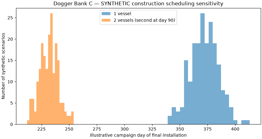
Common random weather is used in both alternatives to isolate vessel count. Uncertainty bands represent variation under this invented weather law, NOT probabilities about actual Dogger Bank construction.
scenarios = []
for run in range(ENSEMBLE_SIZE):
    workable = weather_scenario(ENSEMBLE_SEED + run)
    baseline = simulate_installation(
        PHASE_TURBINES,
        vessel_start_days=(0,),
        workable_days=workable,
        workable_days_per_turbine=WORKABLE_DAYS_PER_TURBINE,
    )
    second_vessel = simulate_installation(
        PHASE_TURBINES,
        vessel_start_days=(0, SECOND_VESSEL_DAY),
        workable_days=workable,
        workable_days_per_turbine=WORKABLE_DAYS_PER_TURBINE,
    )
    scenarios.append((baseline, second_vessel))

one_vessel_days = np.array([a.duration_days for a, _ in scenarios])
two_vessel_days = np.array([b.duration_days for _, b in scenarios])
saved_days = one_vessel_days - two_vessel_days

print("SOURCE FACTS (project announcement):", SOURCE_FACTS)
print("SYNTHETIC assumptions: 70% daily workability; 3 workable days/turbine")
print("SYNTHETIC arrival offset: 90 campaign days (not Q3 start-date inference)")
print("SYNTHETIC one-vessel median completion:", float(np.median(one_vessel_days)))
print("SYNTHETIC two-vessel median completion:", float(np.median(two_vessel_days)))
print("SYNTHETIC saved campaign days, P10/P50/P90:", np.percentile(saved_days, [10, 50, 90]))

fig, ax = plt.subplots(figsize=(8.5, 4.5), layout="constrained")
ax.hist(one_vessel_days, bins=20, alpha=0.6, label="1 vessel")
ax.hist(two_vessel_days, bins=20, alpha=0.6, label="2 vessels (second at day 90)")
ax.set(
    title="Dogger Bank C — SYNTHETIC construction scheduling sensitivity",
    xlabel="Illustrative campaign day of final installation",
    ylabel="Number of synthetic scenarios",
)
ax.legend()
plt.show()
SOURCE FACTS (project announcement): {'turbines': 87, 'capacity_mw': 1200.0, 'second_vessel_arrival_window': 'Q3 2027', 'published_on': '2026-11-04', 'source': 'https://doggerbank.com/news/'}
SYNTHETIC assumptions: 70% daily workability; 3 workable days/turbine
SYNTHETIC arrival offset: 90 campaign days (not Q3 start-date inference)
SYNTHETIC one-vessel median completion: 372.0
SYNTHETIC two-vessel median completion: 232.0
SYNTHETIC saved campaign days, P10/P50/P90: [130.  139.5 152. ]
3. Grid-connection sensitivity: what if completion is not the critical path?#
Potential generation assumes each equal-rated turbine can export no earlier than the day after installation plus a common grid-ready date; constant net capacity factor is illustrative. Grid readiness at day 350 can erase much of the benefit of accelerating installation if both finish beforehand.
fig, ax = plt.subplots(figsize=(8.5, 4.5), layout="constrained")
for grid_ready_day in (0, 350, 500):
    energy_advantages = []
    for one, two in scenarios:
        params = dict(
            project_capacity_mw=PHASE_CAPACITY_MW,
            net_capacity_factor=NET_CAPACITY_FACTOR,
            horizon_days=DAYS,
            grid_ready_day=grid_ready_day,
        )
        one_mwh = commissioning_opportunity_mwh(one, **params)
        two_mwh = commissioning_opportunity_mwh(two, **params)
        energy_advantages.append(max(0.0, two_mwh - one_mwh))
    low, middle, high = np.percentile(energy_advantages, [10, 50, 90])
    print(
        f"ILLUSTRATIVE grid-ready day {grid_ready_day}: additional energy opportunity "
        f"P10/P50/P90 {low:,.0f}/{middle:,.0f}/{high:,.0f} MWh; "
        f"median gross value at a HYPOTHETICAL €65/MWh: "
        f"€{middle * ASSUMED_PRICE_EUR_MWH:,.0f}"
    )
    ax.errorbar(
        grid_ready_day,
        middle,
        yerr=[[middle - low], [high - middle]],
        marker="o",
        capsize=5,
        label=f"Grid day {grid_ready_day}",
    )
ax.set(
    title="Additional modeled energy opportunity, NOT actual generation or revenue",
    xlabel="SYNTHETIC common grid-ready campaign day",
    ylabel="Additional potential exported energy by day 560 (MWh)",
)
ax.set_xlim(-45, 545)
ax.grid(alpha=0.2)
plt.show()
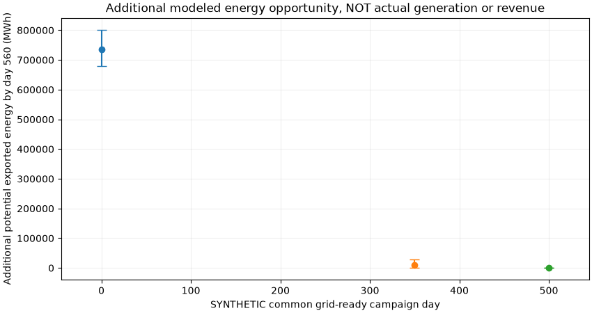
ILLUSTRATIVE grid-ready day 0: additional energy opportunity P10/P50/P90 680,252/735,691/801,887 MWh; median gross value at a HYPOTHETICAL €65/MWh: €47,819,917
ILLUSTRATIVE grid-ready day 350: additional energy opportunity P10/P50/P90 953/10,646/27,521 MWh; median gross value at a HYPOTHETICAL €65/MWh: €691,994
ILLUSTRATIVE grid-ready day 500: additional energy opportunity P10/P50/P90 0/0/0 MWh; median gross value at a HYPOTHETICAL €65/MWh: €0
The plotted P10/P90 intervals ONLY reflect the invented independent-day weather process. They are not a confidence interval for this project. This model excludes port/logistics, foundation readiness, vessel capabilities, turbine-specific ratings, cable commissioning, contractual delay penalties, downtime correlation, electricity market prices and O&M costs. A real financial case requires validated site progress, metocean and grid schedules.
Total running time of the script: (0 minutes 0.228 seconds)