Note
Go to the end to download the full example code.
India BESS policy: evening peak-shifting storage sizing (synthetic study)#
India announced plans to require electricity buyers, including state utilities, to install storage (Reuters, 5 November 2026). The required size was not specified. Its cabinet approved a ₹145 billion storage programme on 4 November. News: https://www.reuters.com/business/energy/india-mandate-energy-storage-state-power-utilities-power-secretary-says-2026-11-05/
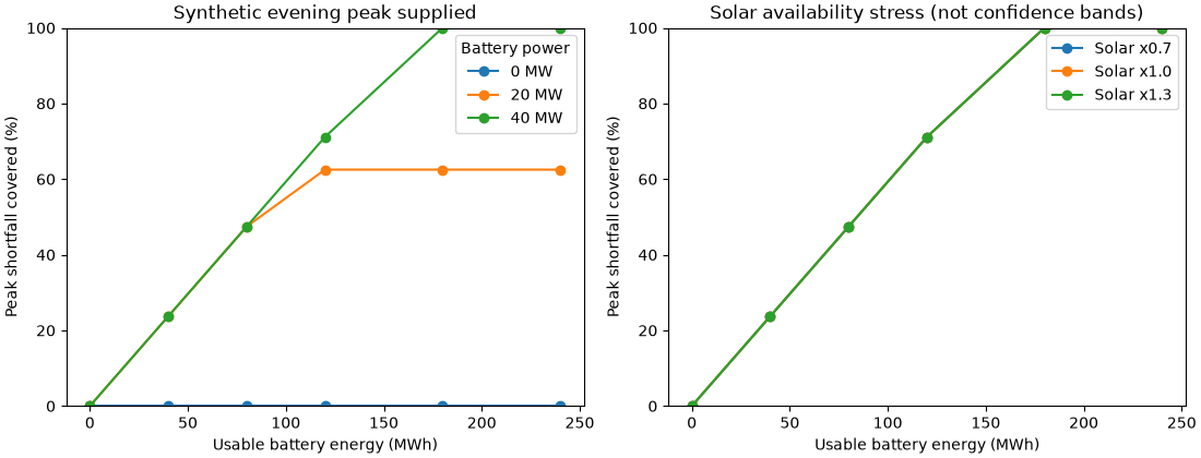
Business question: How do usable BESS energy and power affect the fraction of residual evening peak supplied from otherwise-surplus daytime PV?
Data: This is a fully SYNTHETIC, deterministic seven-day illustration at an arbitrary 100-MW-class system scale. No actual Indian dispatch, load, weather or mandated storage size is inferred. Solar availability stress cases are sensitivity scenarios, not probabilistic uncertainty intervals.
Method: Solar surplus after contemporaneous load charges the battery.
Evening deficit later discharges it, respecting MW/MWh and 90% round-trip loss.
No-storage is the physical baseline. No grid charging or market prices.
See docs/india-storage-peak-shift.md for limitations and reproduction.
import math

import matplotlib.pyplot as plt

from energy_methods.storage_peak_shift import simulate_storage_peak_shift

hours = list(range(7 * 24))
# Every input below is SYNTHETIC, not observations or a published India series.
# Solar surplus after contemporaneous load; peak shortfall 18:00-22:00.
solar_surplus = [max(0.0, 64 * math.sin(math.pi * ((h % 24) - 6) / 12) - 18) for h in hours]
peak_shortfall = [32.0 if 18 <= h % 24 < 23 else 0.0 for h in hours]

powers_mw = [0.0, 20.0, 40.0]
energies_mwh = [0.0, 40.0, 80.0, 120.0, 180.0, 240.0]
solar_factors = (0.7, 1.0, 1.3)

fig, axes = plt.subplots(1, 2, figsize=(11, 4.2), layout="constrained")
for power in powers_mw:
    coverage = []
    for capacity in energies_mwh:
        result = simulate_storage_peak_shift(
            solar_surplus,
            peak_shortfall,
            battery_power_mw=power,
            battery_energy_mwh=capacity,
        )
        coverage.append(100 * result.peak_coverage)
    axes[0].plot(energies_mwh, coverage, marker="o", label=f"{power:.0f} MW")
axes[0].set(
    title="Synthetic evening peak supplied",
    xlabel="Usable battery energy (MWh)",
    ylabel="Peak shortfall covered (%)",
    ylim=(0, 100),
)
axes[0].legend(title="Battery power")

for factor in solar_factors:
    coverage = []
    for capacity in energies_mwh:
        result = simulate_storage_peak_shift(
            [factor * value for value in solar_surplus],
            peak_shortfall,
            battery_power_mw=40,
            battery_energy_mwh=capacity,
        )
        coverage.append(100 * result.peak_coverage)
    axes[1].plot(energies_mwh, coverage, marker="o", label=f"Solar x{factor:.1f}")
axes[1].set(
    title="Solar availability stress (not confidence bands)",
    xlabel="Usable battery energy (MWh)",
    ylabel="Peak shortfall covered (%)",
    ylim=(0, 100),
)
axes[1].legend()
plt.show()
Auditable one-day state of charge and peak delivery for the illustrative 40-MW / 120-MWh case. SOC starts at zero before the first day.
selected = simulate_storage_peak_shift(
    solar_surplus,
    peak_shortfall,
    battery_power_mw=40,
    battery_energy_mwh=120,
)
base = simulate_storage_peak_shift(
    solar_surplus,
    peak_shortfall,
    battery_power_mw=0,
    battery_energy_mwh=0,
)
print(f"SYNTHETIC no-storage evening shortfall: {base.peak_shortfall_mwh:.1f} MWh")
print(f"SYNTHETIC 40 MW / 120 MWh: delivered {selected.peak_delivered_mwh:.1f} MWh")
print(f"SYNTHETIC coverage: {selected.peak_coverage:.1%}")
print(f"SYNTHETIC curtailed surplus: {selected.curtailed_mwh:.1f} MWh")
fig, ax = plt.subplots(layout="constrained")
ax.step(
    range(24),
    [step.soc_mwh for step in selected.steps[:24]],
    where="mid",
)
ax.set(
    xlabel="Synthetic day-1 hour",
    ylabel="Usable state of charge (MWh)",
    title="Daytime renewable charging → evening discharge",
)
ax.set_xlim(0, 23)
plt.show()
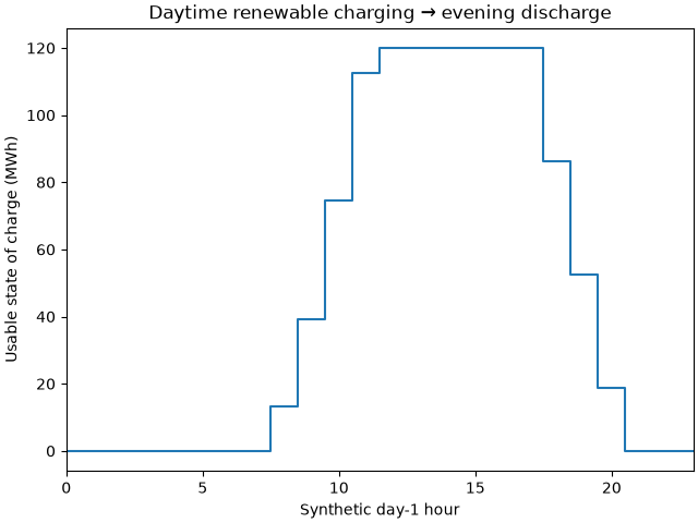
SYNTHETIC no-storage evening shortfall: 1120.0 MWh
SYNTHETIC 40 MW / 120 MWh: delivered 796.9 MWh
SYNTHETIC coverage: 71.2%
SYNTHETIC curtailed surplus: 1151.6 MWh
Reproduce: uv run –no-sync python examples/analysis/plot_india_storage_mandate.py The stress curves are engineering sensitivity, not an India storage forecast.
Total running time of the script: (0 minutes 0.205 seconds)