Note
Go to the end to download the full example code.
Solar farm near Candelaria: Icor, Tenerife#
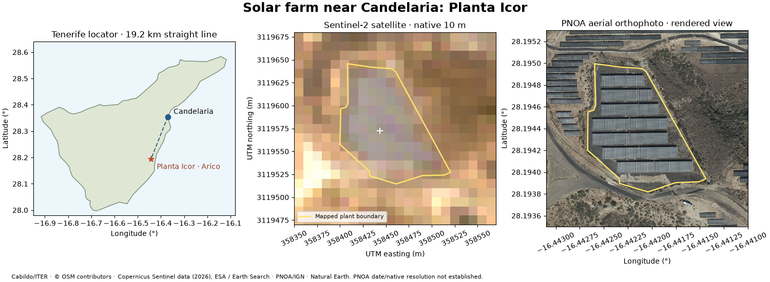
Locate Planta Icor, a ground-mounted PV installation in Arico, about 19.2 km south of Candelaria in a straight line. It is not in Candelaria municipality and this is not a nearest-farm search. The Cabildo de Tenerife / ITER catalogue supplies the name, coordinates and listed 2,000 kW capacity. The capacity is provider metadata; its AC/DC basis is not specified in this dataset.
This example adds a site-level workflow to the earlier general imagery demo: associate the official point with a mapped plant boundary, locate it relative to Candelaria, compare satellite and aerial views, and inspect local quality. The boundary is OpenStreetMap way 430266023, associated by point-in-polygon; that association is not a survey or an operator-validated site boundary.
Run with Python 3.13 and the optional imagery workspace group. Download
the complete script, images and metadata.
See the imagery guide for
installation and live connector usage. This gallery runs entirely offline.
Continue with automatic module counting for an annotated candidate count from the detailed aerial image.
Credits: Cabildo de Tenerife / ITER (CC BY), OpenStreetMap contributors (ODbL), Copernicus Sentinel data (2026) / ESA / Element 84, PNOA/IGN and Natural Earth.
import hashlib
import json
from dataclasses import asdict
from pathlib import Path

import matplotlib.pyplot as plt
import numpy as np
from matplotlib.colors import BoundaryNorm, ListedColormap
from pyproj import Geod, Transformer
from rasterio import Affine
from rasterio.features import geometry_mask
from shapely import transform
from shapely.geometry import mapping, shape

from energy_data_retrieval.sources.orbitalpv_imagery import describe_asset, load_satellite_image

DATA = (
    Path(globals().get("__file__", Path.cwd() / "plot_candelaria_solar_farm.py")).resolve().parent
    / "data"
)
site = json.loads((DATA / "candelaria_site.json").read_text())
official = site["official_site"]
point = shape(official["geometry"])
footprint = shape(site["footprint"]["geometry"])
assert footprint.covers(point)
town = site["candelaria_reference_lonlat"]
distance_km = Geod(ellps="WGS84").inv(*town, point.x, point.y)[2] / 1000
visual = load_satellite_image(str(DATA / "candelaria_visual.tif"))
red = load_satellite_image(str(DATA / "candelaria_red.tif"))
scl = load_satellite_image(str(DATA / "candelaria_scl.tif"))
pnoa_path = DATA / site["aerial_fixture"]
pnoa_meta = json.loads(pnoa_path.with_suffix(".png.meta.json").read_text())
assert hashlib.sha256(pnoa_path.read_bytes()).hexdigest() == pnoa_meta["sha256"]
assert pnoa_meta["product_kind"] == "rendered_display"
1. Locate the farm and preserve the distinction between image products#
A finer WMS image width is not evidence of finer native sensor resolution. Sentinel-2 is a native 10 m satellite crop acquired on 4 August 2026. PNOA is rendered aerial orthophotography; this request does not establish the source capture date or native resolution. These images are not a change-detection pair.
project = Transformer.from_crs(4326, visual.crs, always_xy=True)
outline = transform(footprint, project.transform, interleaved=False)
east, north = project.transform(point.x, point.y)


def satellite(ax, image, values, title, **kwargs):
    left, bottom, right, top = image.bounds
    artist = ax.imshow(
        values,
        extent=(left, right, bottom, top),
        origin="upper",
        interpolation="nearest",
        **kwargs,
    )
    ax.plot(*outline.exterior.xy, color="#ffe36b", lw=1.8, label="Mapped plant boundary")
    ax.set(title=title, xlabel="UTM easting (m)", ylabel="UTM northing (m)")
    ax.ticklabel_format(style="plain", useOffset=False)
    ax.tick_params(axis="x", rotation=25)
    return artist


rgb = np.moveaxis(visual.data.filled(0), 0, -1).astype(float) / 255
alpha = (~np.ma.getmaskarray(visual.data).any(axis=0)).astype(float)
fig_location, axes = plt.subplots(1, 3, figsize=(15, 5.5), layout="constrained")
island = shape(json.loads((DATA / "candelaria_tenerife.geojson").read_text())["geometry"])
axes[0].fill(*island.exterior.xy, facecolor="#dfe7d4", edgecolor="#768973", lw=1)
axes[0].set_facecolor("#edf6fb")
axes[0].plot([town[0], point.x], [town[1], point.y], "--", color="#426a89", lw=1.5)
axes[0].scatter(*town, s=55, color="#205c87", zorder=4)
axes[0].scatter(point.x, point.y, s=70, color="#c44831", marker="*", zorder=4)
axes[0].annotate("Candelaria", town, xytext=(8, 4), textcoords="offset points", fontsize=10)
axes[0].annotate(
    "Planta Icor · Arico",
    (point.x, point.y),
    xytext=(8, -14),
    textcoords="offset points",
    fontsize=10,
    color="#963824",
)
axes[0].set(
    title=f"Tenerife locator · {distance_km:.1f} km straight line",
    xlabel="Longitude (°)",
    ylabel="Latitude (°)",
    xlim=(-16.95, -16.08),
    ylim=(27.98, 28.64),
)
axes[0].set_aspect(1 / np.cos(np.deg2rad(28.3)))
satellite(axes[1], visual, np.dstack((rgb, alpha)), "Sentinel-2 satellite · native 10 m")
axes[1].scatter(east, north, marker="+", s=80, color="white", linewidth=1.5)
axes[1].legend(loc="lower left", fontsize=8)
west, south, east_lon, north_lat = pnoa_meta["bbox_wgs84"]
axes[2].imshow(
    plt.imread(pnoa_path),
    extent=(west, east_lon, south, north_lat),
    origin="upper",
    interpolation="nearest",
)
axes[2].plot(*footprint.exterior.xy, color="#ffe36b", lw=1.8)
axes[2].set_aspect(1 / np.cos(np.deg2rad(point.y)))
axes[2].set(
    title="PNOA aerial orthophoto · rendered view", xlabel="Longitude (°)", ylabel="Latitude (°)"
)
axes[2].ticklabel_format(style="plain", useOffset=False)
axes[2].tick_params(axis="x", rotation=25)
fig_location.suptitle("Solar farm near Candelaria: Planta Icor", fontsize=18, weight="bold")
fig_location.text(
    0.015,
    0.012,
    "Cabildo/ITER · © OSM contributors · Copernicus Sentinel data (2026), ESA / Earth Search · "
    "PNOA/IGN · Natural Earth. "
    "PNOA date/native resolution not established.",
    fontsize=8,
)

fig_location.set_layout_engine("constrained", rect=(0, 0.065, 1, 0.935))
2. Inspect calibrated reflectance and local scene quality#
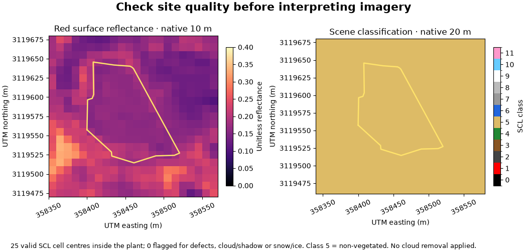
Each layer keeps its original grid. Cell centres inside the mapped footprint define the summary, so boundary pixels can mix panels and surrounding land. At 20 m the SCL sample is small. Clear classifications are useful screening, not proof that every panel is visible or that the plant is operating normally.
scl_project = Transformer.from_crs(4326, scl.crs, always_xy=True)
scl_outline = transform(footprint, scl_project.transform, interleaved=False)
inside = geometry_mask(
    [mapping(scl_outline)],
    out_shape=scl.data.shape[1:],
    transform=Affine(*scl.transform),
    invert=True,
    all_touched=False,
)
valid = inside & ~np.ma.getmaskarray(scl.data[0])
classes, counts = np.unique(scl.data[0].data[valid], return_counts=True)
class_counts = {int(k): int(v) for k, v in zip(classes, counts, strict=True)}
problem_pixels = int(np.isin(scl.data[0].data[valid], [0, 1, 3, 8, 9, 10, 11]).sum())
fig_quality, axes = plt.subplots(1, 2, figsize=(10.5, 5), layout="constrained")
artist = satellite(
    axes[0],
    red,
    red.reflectance()[0],
    "Red surface reflectance · native 10 m",
    cmap="magma",
    vmin=0,
    vmax=0.4,
)
fig_quality.colorbar(artist, ax=axes[0], shrink=0.7, label="Unitless reflectance")
cmap = ListedColormap(
    [
        "black",
        "red",
        "#444444",
        "#885522",
        "#228833",
        "#ddbb66",
        "#2266dd",
        "#999999",
        "#bbbbbb",
        "white",
        "#66ccff",
        "#ff99cc",
    ]
)
artist = satellite(
    axes[1],
    scl,
    scl.data[0],
    "Scene classification · native 20 m",
    cmap=cmap,
    norm=BoundaryNorm(np.arange(-0.5, 12.5), 12),
)
fig_quality.colorbar(artist, ax=axes[1], shrink=0.7, ticks=range(12), label="SCL class")
fig_quality.suptitle("Check site quality before interpreting imagery", fontsize=16, weight="bold")
fig_quality.text(
    0.02,
    0.012,
    f"{int(valid.sum())} valid SCL cell centres inside the plant; {problem_pixels} flagged for "
    "defects, cloud/shadow or snow/ice. Class 5 = non-vegetated. No cloud removal applied.",
    fontsize=9,
)

fig_quality.set_layout_engine("constrained", rect=(0, 0.075, 1, 0.925))
3. Read the metadata and decide what to use it for#
The full STAC item and asset definitions remain in image.item_metadata
and image.asset_metadata and in the TIFF’s checksum sidecar. Read dates,
CRS, masks, calibration and resolution before combining other datasets.
summary = {
    "site": official["properties"],
    "longitude_latitude": next(iter(point.coords)),
    "distance_from_candelaria_km": round(distance_km, 3),
    "osm_plant_way": site["footprint"]["properties"]["osm_id"],
    "mapped_boundary_area_ha": round(outline.area / 10_000, 3),
    "boundary_interpretation": "Mapped site area, not panel surface area or surveyed ownership",
    "satellite": asdict(describe_asset(visual.item_metadata, "visual")),
    "satellite_scene_cloud_percent": visual.item_metadata["properties"].get("eo:cloud_cover"),
    "scl_inside_plant_counts": class_counts,
    "aerial_product_kind": pnoa_meta["product_kind"],
    "aerial_capture_date": pnoa_meta["acquisition_date"],
    "aerial_native_resolution_m": pnoa_meta["native_resolution_m"],
}
print(json.dumps(summary, indent=2, ensure_ascii=False))
{
  "site": {
    "instalacion_id": 6,
    "instalacion_nombre": "Planta Icor",
    "instalacion_tipo": "Fotovoltaica",
    "instalacion_potencia": 2000,
    "instalacion_unidad_potencia": "kW",
    "instalacion_latitud": 28.194341,
    "instalacion_longitud": -16.442229
  },
  "longitude_latitude": [
    -16.442229,
    28.194341
  ],
  "distance_from_candelaria_km": 19.163,
  "osm_plant_way": 430266023,
  "mapped_boundary_area_ha": 0.993,
  "boundary_interpretation": "Mapped site area, not panel surface area or surveyed ownership",
  "satellite": {
    "scene_id": "S2A_T28RCS_20260804T115232_L2A",
    "asset_key": "visual",
    "product_kind": "rendered_rgb",
    "native_gsd_m": 10.0,
    "grid_spacing_m": [
      10.0,
      10.0
    ],
    "detail_limit_m": 10.0,
    "acquisition_utc": "2026-08-04T11:53:59.065000Z",
    "platform": "sentinel-2a"
  },
  "satellite_scene_cloud_percent": 0.155066,
  "scl_inside_plant_counts": {
    "5": 25
  },
  "aerial_product_kind": "rendered_display",
  "aerial_capture_date": "mixed_or_unknown; inspect original metadata",
  "aerial_native_resolution_m": null
}
Use the imagery to check mapped layout and surrounding land. Use the official catalogue to identify the plant and distinguish its listed power from a prediction. Use the separate PVGIS and terrain connectors for modelled yield and terrain context at these coordinates. The images do not measure output, module health or degradation, and the 2,000 kW field does not establish a DC peak-power input without checking the plant’s technical records.
plt.show()
Total running time of the script: (0 minutes 0.716 seconds)