Note
Go to the end to download the full example code.
Mistral Timestral: a day-ahead solar and wind forecast#
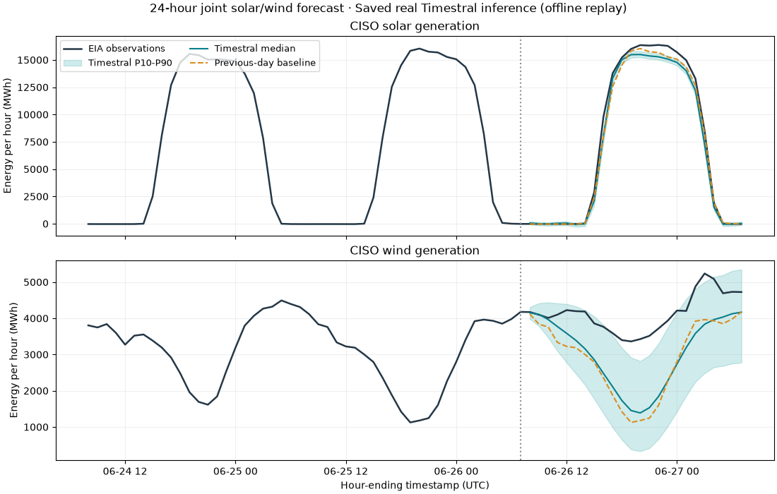
Forecast 24 hours of California ISO solar and wind generation jointly, using six days of attributed EIA-930 observations. The gallery replays real saved Timestral-5M inference, then recalculates metrics and plots offline. It does not download model weights or require PyTorch during documentation builds.
To rerun actual inference, install the optional official Timestral package and
set ENERGY_TIMESTRAL_LIVE=1. The script uses the exact checkpoint revision
from its manifest and fails on inference errors; it never substitutes a baseline.
See the Timestral guide for setup.
Download this example with its data, the
forecast provenance, or the
saved quantiles.
Scope: system-level hourly energy in MWh, not a solar farm forecast. One historical holdout is not proof of operational forecasting skill. Pretraining overlap is unknown, and the model’s prediction bands are not calibrated here.
1. Load verified observations and a chronological holdout#
EIA timestamps mark the end of each UTC hour. The first 144 hours are the context; the final 24 hours are held out. Only the UTC clock’s sine and cosine are supplied as known-future covariates. No future observed weather or target generation enters the forecast.
import json
import os
from pathlib import Path

import matplotlib.pyplot as plt

from energy_analysis.timestral_case import (
    FUEL_TYPES,
    HORIZON,
    PROVENANCE_NAME,
    evaluate_timestral_case,
    forecast_timestral_case,
    load_timestral_case,
    load_timestral_snapshot,
)
from energy_methods.timestral import TimestralConnector

example_directory = (
    Path(globals().get("__file__", Path.cwd() / "plot_timestral_forecast.py")).resolve().parent
)
data_directory = example_directory / "data"
case = load_timestral_case(data_directory)
manifest = json.loads((data_directory / PROVENANCE_NAME).read_text())
print(f"Model: {manifest['model_id']} @ {manifest['model_revision']}")
print(f"Context: {case.context.shape[-1]} hours; holdout: {HORIZON} hours")
Model: mistralai/Timestral-5M @ bdd20cfc15a3fea0e4cb5ccef37f8d3ca7aa335f
Context: 144 hours; holdout: 24 hours
2. Replay the captured model forecast, or explicitly run inference#
Input/output checksums prevent displaying a stale forecast against changed
data. Live execution can use ENERGY_TIMESTRAL_DEVICE=cuda; default is CPU.
Use ENERGY_TIMESTRAL_LOCAL_ONLY=1 to forbid new checkpoint downloads.
if os.environ.get("ENERGY_TIMESTRAL_LIVE") == "1":
    connector = TimestralConnector(
        manifest["model_id"],
        revision=manifest["model_revision"],
        device=os.environ.get("ENERGY_TIMESTRAL_DEVICE", "cpu"),
        local_files_only=os.environ.get("ENERGY_TIMESTRAL_LOCAL_ONLY") == "1",
    )
    forecast = forecast_timestral_case(case, connector)
    mode = "Live Timestral inference"
else:
    forecast = load_timestral_snapshot(data_directory, case)
    mode = "Saved real Timestral inference (offline replay)"
print(mode)
Saved real Timestral inference (offline replay)
3. Plot the medians, model intervals and daily baseline#
P10-P90 is the central 80% model prediction interval. Observed coverage for just 24 hours is descriptive; it is not a calibration guarantee.
future = case.profiles.index[-HORIZON:]
fig, axes = plt.subplots(2, 1, figsize=(11, 7), layout="constrained", sharex=True)
for i, (fuel, label) in enumerate(zip(FUEL_TYPES, ("Solar", "Wind"), strict=True)):
    ax = axes[i]
    ax.plot(
        case.profiles.index[-72:],
        case.profiles[fuel].iloc[-72:],
        color="#243746",
        label="EIA observations",
        linewidth=1.8,
    )
    ax.fill_between(
        future,
        forecast.quantile(0.1)[0, i],
        forecast.quantile(0.9)[0, i],
        color="#149b9b",
        alpha=0.2,
        label="Timestral P10-P90",
    )
    ax.plot(future, forecast.median[0, i], color="#087e8b", label="Timestral median")
    ax.plot(
        future,
        case.context[0, i, -HORIZON:],
        color="#d98e21",
        linestyle="--",
        label="Previous-day baseline",
    )
    ax.axvline(case.profiles.index[-HORIZON - 1], color="#8a929a", linestyle=":")
    ax.set(title=f"CISO {label.lower()} generation", ylabel="Energy per hour (MWh)")
    ax.grid(alpha=0.2)
axes[0].legend(ncols=2, fontsize=9, loc="upper left")
axes[-1].set_xlabel("Hour-ending timestamp (UTC)")
fig.suptitle(f"24-hour joint solar/wind forecast · {mode}", fontsize=12)
plt.show()
4. Compare with both simple baselines#
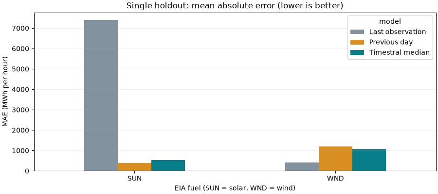
WAPE divides total absolute error by the sum of absolute observed energy. All 24 hours count, including zeros and EIA’s negative nighttime net generation. The model may lose to a baseline. These results do not justify a broad claim about Timestral’s accuracy across sites, seasons or technologies.
metrics = evaluate_timestral_case(case, forecast)
print(metrics.round(3).to_string(index=False))
fig, ax = plt.subplots(figsize=(9, 4), layout="constrained")
metrics.pivot(index="fuel", columns="model", values="mae_mwh").plot.bar(
    ax=ax, rot=0, color=["#82929e", "#d98e21", "#087e8b"]
)
ax.set(
    title="Single holdout: mean absolute error (lower is better)",
    xlabel="EIA fuel (SUN = solar, WND = wind)",
    ylabel="MAE (MWh per hour)",
)
ax.grid(axis="y", alpha=0.2)
plt.show()
           model fuel  hours  mae_mwh  rmse_mwh  wape_pct  p10_p90_coverage
Timestral median  SUN     24  533.723   737.141     7.215             0.458
Timestral median  WND     24 1078.922  1242.178    26.074             0.583
    Previous day  SUN     24  389.583   606.637     5.266               NaN
    Previous day  WND     24 1207.375  1364.347    29.178               NaN
Last observation  SUN     24 7402.833 10360.732   100.073               NaN
Last observation  WND     24  407.208   520.845     9.841               NaN
Total running time of the script: (0 minutes 0.264 seconds)