Note
Go to the end to download the full example code.
Japan: three days of real Tokyo-area generation#
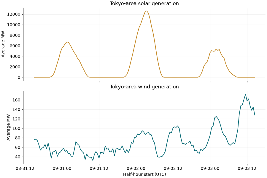
Parse TEPCO Power Grid’s actual/estimated generation mix for 1-3 September 2026. The source CSV explicitly declares half-hour average MW. The 144 observations are genuine public rows, transcoded from CP932 to UTF-8 without changing their values. Source and subset checksums are preserved.
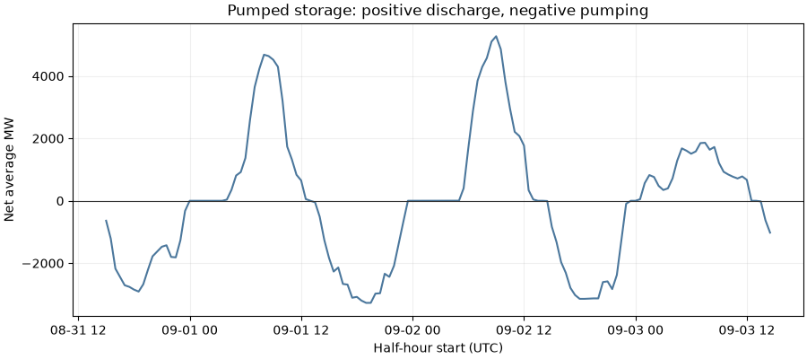
This is the Tokyo service area’s technology mix. Some values are publisher estimates and retrospective revisions are possible. Storage, curtailment and interconnector flows remain separately labelled rather than added to generation. See TEPCO’s definitions and monthly files.
Download the real CSV and
provenance alongside this script,
keeping them in a data/ subdirectory. No network or key is used here.
import hashlib
import json
from pathlib import Path

import matplotlib.pyplot as plt

from energy_data_retrieval.sources.tepco import parse_generation_csv
1. Verify the captured observations and their declared units#
directory = (
    Path(globals().get("__file__", Path.cwd() / "plot_generation_tepco.py")).resolve().parent
)
data = directory / "data"
raw = (data / "generation_tepco.csv").read_bytes()
manifest = json.loads((data / "generation_tepco_provenance.json").read_text())
if hashlib.sha256(raw).hexdigest() != manifest["fixture_sha256"]:
    raise ValueError("TEPCO sample differs from its acquisition manifest")
frame = parse_generation_csv(raw, include_flows=True)
print("Source:", manifest["source_url"])
print(frame[["source_unit", "unit", "flow"]].drop_duplicates())
Source: https://www.tepco.co.jp/forecast/html/images/eria_jukyu_202609_03.csv
   source_unit unit         flow
0           MW   MW  curtailment
2           MW   MW   generation
13          MW   MW   net_import
14          MW   MW  storage_net
2. Compare solar and wind without changing MW into MWh#
generation = frame.loc[frame.flow.eq("generation")]
fig, axes = plt.subplots(2, 1, figsize=(9, 6), sharex=True, layout="constrained")
for ax, technology, color in zip(axes, ["solar", "wind"], ["#c48a28", "#096b76"], strict=True):
    observations = generation.loc[generation.technology.eq(technology)]
    ax.plot(observations.timestamp, observations.value, color=color)
    ax.set(ylabel="Average MW", title=f"Tokyo-area {technology} generation")
    ax.grid(alpha=0.2)
axes[-1].set_xlabel("Half-hour start (UTC)")
plt.show()
3. Show signed storage separately from generation#
storage = frame.loc[frame.technology.eq("pumped_storage")]
fig, ax = plt.subplots(figsize=(9, 4), layout="constrained")
ax.plot(storage.timestamp, storage.value, color="#4b779c")
ax.axhline(0, color="#333333", linewidth=0.8)
ax.set(
    xlabel="Half-hour start (UTC)",
    ylabel="Net average MW",
    title="Pumped storage: positive discharge, negative pumping",
)
ax.grid(alpha=0.2)
plt.show()
4. Convert only the generation intervals to energy#
Each record covers 0.5 hours; totals below are over the three captured days.
energy = generation.groupby("technology").value.sum(min_count=1) * 0.5
print("Three-day energy by technology (MWh):")
print(energy.round(1))
Three-day energy by technology (MWh):
technology
biomass            39933.5
coal              546861.0
geothermal             0.0
hydro             120800.5
lng              1016269.5
nuclear            92914.5
oil                22381.0
other              21727.0
other_thermal     118498.0
solar             158109.5
wind                5188.0
Name: value, dtype: float64
Total running time of the script: (0 minutes 0.241 seconds)