Note
Go to the end to download the full example code.
New Zealand: real solar, wind and hydro across a clock change#
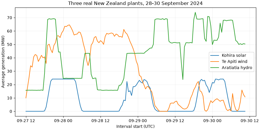
Read actual Electricity Authority metered-injection observations associated with three New Zealand plants, 28-30 September 2024. The middle day has 46 half-hour trading periods because daylight saving starts. This is an offline example using unchanged source CSV rows with provenance and checksums.
EMI maps metered injections to plants; some shared points are apportioned. These are kWh per trading period, not direct unit SCADA or instantaneous MW. See the official dataset and definitions. Attribution: Electricity Authority (New Zealand), CC-BY 4.0.
Download the real CSV and
provenance alongside this script,
keeping them in a data/ subdirectory.
import hashlib
import json
from pathlib import Path

import matplotlib.pyplot as plt

from energy_data_retrieval.sources.emi import parse_generation_csv
1. Verify the attributed capture#
directory = Path(globals().get("__file__", Path.cwd() / "plot_generation_emi.py")).resolve().parent
data = directory / "data"
raw = (data / "generation_emi.csv").read_bytes()
manifest = json.loads((data / "generation_emi_provenance.json").read_text())
if hashlib.sha256(raw).hexdigest() != manifest["fixture_sha256"]:
    raise ValueError("EMI sample differs from its acquisition manifest")
print("Source:", manifest["source_url"])
Source: https://emidatasets.blob.core.windows.net/publicdata/Datasets/Wholesale/Generation/Generation_MD/202409_Generation_MD.csv
2. Normalize real intervals and inspect the clock-change day#
frame = parse_generation_csv(raw)
print(frame.groupby(["plant_id", "source_date"]).size().unstack())
print("UTC half-hour records:", len(frame))
source_date  2024-09-28  2024-09-29  2024-09-30
plant_id
Kohira               48          46          48
aratiatia            48          46          48
te_apiti             48          46          48
UTC half-hour records: 426
3. Compare plant profiles with an explicit energy-to-power conversion#
One half hour of kWh divided by 500 gives its average MW. This conversion uses actual interval lengths and does not invent missing observations.
fig, ax = plt.subplots(figsize=(9, 4.5), layout="constrained")
for plant, label in (
    ("Kohira", "Kohira solar"),
    ("te_apiti", "Te Apiti wind"),
    ("aratiatia", "Aratiatia hydro"),
):
    values = frame.loc[frame.plant_id.eq(plant)]
    ax.plot(values.timestamp, values.value / 500, label=label)
ax.set(
    xlabel="Interval start (UTC)",
    ylabel="Average generation (MW)",
    title="Three real New Zealand plants, 28-30 September 2024",
)
ax.grid(alpha=0.2)
ax.legend()
plt.show()
4. Aggregate energy without assuming every day has 48 observations#
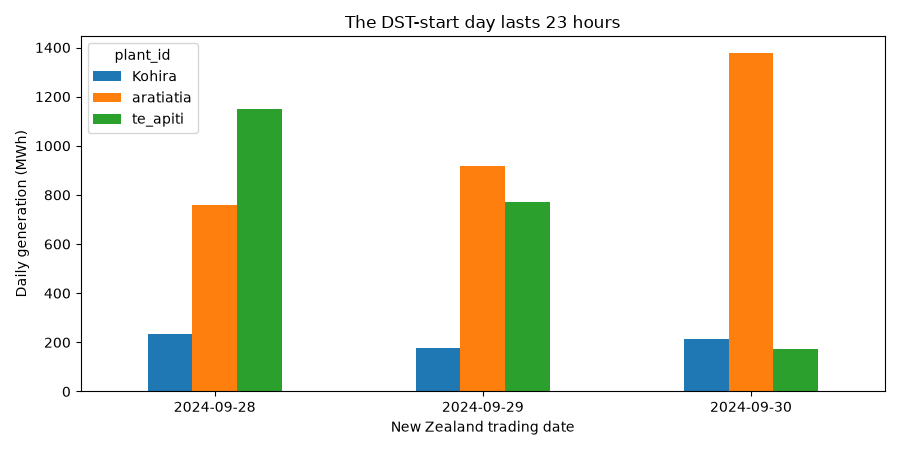
daily = frame.groupby(["source_date", "plant_id"]).value.sum(min_count=1).unstack() / 1000
daily.plot.bar(
    figsize=(9, 4.5),
    rot=0,
    ylabel="Daily generation (MWh)",
    xlabel="New Zealand trading date",
    title="The DST-start day lasts 23 hours",
)
plt.tight_layout()
plt.show()
Total running time of the script: (0 minutes 0.186 seconds)