Note
Go to the end to download the full example code.
Map one country or a group of countries#
Use detailed Natural Earth 1:10 million country contours to clip maps for Austria and Slovenia, then zoom to Slovenia alone. The input fixture contains real 2023 weather on a 0.5° sampling grid, independently acquired from NASA POWER and Open-Meteo ERA5-Land. It is not an upsampled version of the 15° worldwide example. AOD retains its 1° source support; finer plotting cannot add aerosol information. The snow samples use the explicitly selected model’s nearest cells. This single-year example remains empirical screening.
Download the inputs,
provenance and
country contours alongside this
script. The contours are an unsimplified subset of the retrieved shapefile.
Run offline from the repository’s examples/analysis directory. See
the country mapping guide for
shapefile acquisition/export, country names/codes, grid spacing and map bounds.
import hashlib
import json
from pathlib import Path

import matplotlib.pyplot as plt
import numpy as np
import pandas as pd
from matplotlib.colors import BoundaryNorm, ListedColormap
from matplotlib.patches import Patch

from energy_methods.country_boundaries import load_country_boundaries, write_country_boundaries
from energy_methods.country_mapping import (
    clip_country_grid,
    plot_country_map,
    write_country_geojson,
)
from energy_methods.weather_risk import RISK_LABELS
from energy_methods.weather_risk_mapping import map_weather_risks
Load the finer inputs and actual country contours#
Checksums tie the data and boundary subset to the acquisition manifest.
The loader accepts .shp with its companions or WGS84 GeoJSON. Exact names
and codes are case-insensitive; unknown/ambiguous selections raise an error.
provenance = json.loads(Path("country_risk_provenance.json").read_text(encoding="utf-8"))
for filename, checksum in (
    ("country_risk_inputs.csv", "fixture_sha256"),
    ("country_risk_boundaries.geojson", "boundary_fixture_sha256"),
):
    if hashlib.sha256(Path(filename).read_bytes()).hexdigest() != provenance[checksum]:
        raise ValueError(f"Fixture checksum mismatch: {filename}")
boundary_path = Path("country_risk_boundaries.geojson")
countries = load_country_boundaries(boundary_path, ["Austria", "Slovenia"])
table = pd.read_csv("country_risk_inputs.csv").set_index(["year", "lat", "lon"]).to_xarray()
table.aod550_mean.attrs = {"units": "1", "wavelength_nm": 550}
table.snow_depth_sum.attrs = {"units": "cm h", "snow_depth_kind": "physical_ground"}
table.attrs = {
    "country_codes": " ".join(countries.codes),
    "grid_degrees": provenance["grid_degrees"],
}
result = map_weather_risks(table)
unique_aod = {(r["aod_sample_latitude"], r["aod_sample_longitude"]) for r in provenance["requests"]}
print(f"Countries: {countries.codes}; grid: {provenance['grid_degrees']}°")
print(f"Snow samples: {provenance['selected_cells']}; unique 1° AOD samples: {len(unique_aod)}")
Countries: ('AUT', 'SVN'); grid: 0.5°
Snow samples: 83; unique 1° AOD samples: 28
Inspect the continuous indicators#
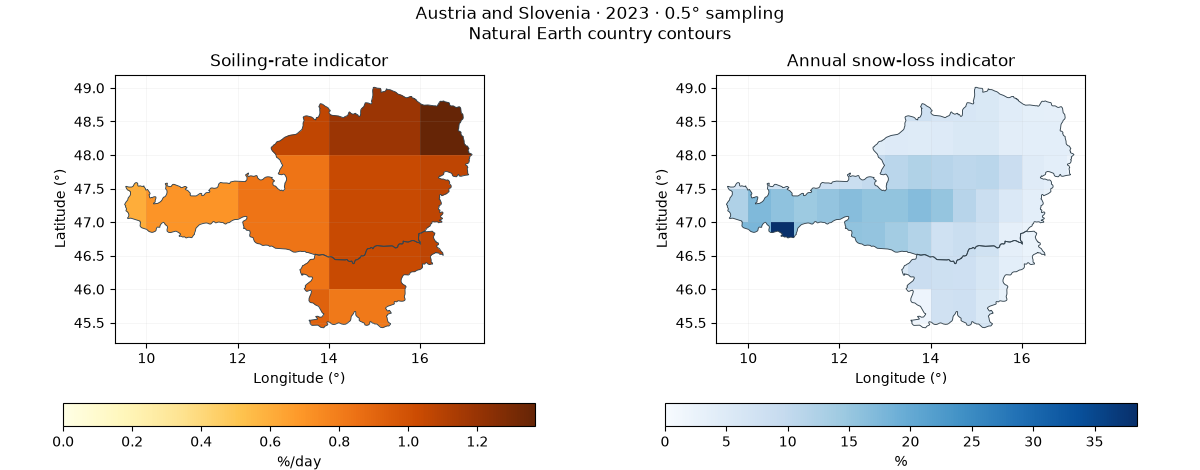
Plot original cell values with flat shading and clip them to the country polygons. Adjacent countries keep their shared border. Country detail comes from the vector contours, while scientific detail comes from the inputs. One requested snow cell is missing; some Alpine source cells report very large annual snow-depth sums. These values are retained for inspection, not independently validated as site losses. All soiling indicators in this sample exceed the thesis’s Very High threshold despite their different magnitudes.
extent = (9.3, 45.2, 17.4, 49.2)
fig, axes = plt.subplots(1, 2, figsize=(12, 4.7), layout="constrained")
for ax, name, title, units, cmap in (
    (axes[0], "soiling_rate", "Soiling-rate indicator", "%/day", "YlOrBr"),
    (axes[1], "snow_loss", "Annual snow-loss indicator", "%", "Blues"),
):
    mesh = plot_country_map(result[name], countries, ax=ax, bounds=extent, cmap=cmap, vmin=0)
    ax.set_title(title)
    fig.colorbar(mesh, ax=ax, orientation="horizontal", shrink=0.8, label=units)
fig.suptitle("Austria and Slovenia · 2023 · 0.5° sampling\nNatural Earth country contours")
plt.show()
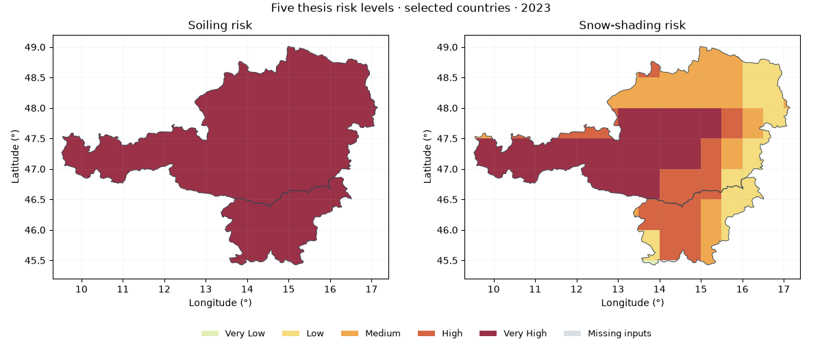
Map both risk categories within the selected countries#
Exact thresholds follow the soiling/snow guide. Categorical IDs are never linearly interpolated. Boundary cells keep their calculated value; their visible footprint is clipped to the country outline. White is outside the selection and gray is missing within the selection.
colors = ["#e3efb9", "#f4dc7f", "#efa950", "#d56543", "#9a3147"]
cmap = ListedColormap(colors)
norm = BoundaryNorm(np.arange(0.5, 6.5), cmap.N)
fig = plt.figure(figsize=(12, 5.2), layout="constrained")
grid = fig.add_gridspec(2, 2, height_ratios=[5, 0.8])
for col, name, title in (
    (0, "soiling_risk", "Soiling risk"),
    (1, "snow_risk", "Snow-shading risk"),
):
    ax = fig.add_subplot(grid[0, col])
    plot_country_map(result[name], countries, ax=ax, bounds=extent, cmap=cmap, norm=norm, nodata=0)
    ax.set_title(title)
legend_ax = fig.add_subplot(grid[1, :])
legend_ax.axis("off")
handles = [
    Patch(facecolor=c, label=label) for c, label in zip(colors, RISK_LABELS[1:], strict=True)
]
handles.append(Patch(facecolor="#d9dfe3", label="Missing inputs"))
legend_ax.legend(handles=handles, ncol=6, frameon=False, loc="center", fontsize=9)
fig.suptitle("Five thesis risk levels · selected countries · 2023")
plt.show()
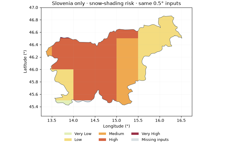
Select a single country from the same inputs#
Masking changes the geographic selection without resampling. This is a zoom, not another increase in weather resolution. The methods also work with KGPV, degradation and other rectilinear latitude/longitude maps.
slovenia = load_country_boundaries(boundary_path, "SVN")
single = clip_country_grid(result.snow_risk, slovenia, nodata=0)
fig, ax = plt.subplots(figsize=(8, 5), layout="constrained")
plot_country_map(
    single, slovenia, ax=ax, bounds=(13.25, 45.25, 16.75, 47), cmap=cmap, norm=norm, nodata=0
)
ax.set_title("Slovenia only · snow-shading risk · same 0.5° inputs")
fig.legend(handles=handles, loc="outside lower center", ncol=3, frameon=False, fontsize=9)
plt.show()
Export selected contours and clipped risk cells#
Shapefile export writes five companion files; move them together. The risk GeoJSON contains country-cell intersections, not full rectangular coastal cells. For area totals, use geodesic or equal-area polygon calculations; counting full intersecting cells overestimates coastal/border area.
export = False
if export:
    output = Path("country-map-output")
    write_country_boundaries(countries, output / "selected_countries.shp")
    write_country_geojson(
        result.snow_risk,
        countries,
        output / "snow_risk.geojson",
        nodata=0,
        labels=dict(enumerate(RISK_LABELS)),
    )
    result.to_netcdf(output / "country_risks.nc")
Source attribution and limits#
Made with Natural Earth: public-domain Admin 0 boundaries at 1:10 million,
default de facto boundary policy. 10m means map scale, not 10-metre
positional accuracy. The original archive version, SHA-256 and selected-file
checksum are in the manifest. NASA POWER/CERES supplies AOD; Open-Meteo
(CC BY 4.0) supplies ERA5-Land snow data. Cite the thesis and method references
in the bibliography.
Total running time of the script: (0 minutes 0.880 seconds)