Note
Go to the end to download the full example code.
STRATA in practice: weather fields to energy-asset scenarios#
How would an analyst connect a completed NVIDIA STRATA rollout to a portfolio of energy assets? This walkthrough exercises the actual output adapter, checks its coordinate and unit conventions, compares paired reference series, and exports auditable scenario results.
All weather, reference values, assets and power plans below are synthetic. No neural-network inference, SCREAM acquisition or real storm forecast occurs. The moving pulse is a teaching fixture on a small STRATA-shaped grid, not a physical atmospheric simulation. The same sampling functions accept real STRATA output; the linked guide supplies the upstream GPU commands and CLI.
See the complete STRATA guide for installation, real-output use, reference preparation, field definitions and limitations.
import matplotlib.pyplot as plt
import numpy as np

from energy_analysis.strata import (
    compare_reference,
    demo_baseline,
    plot_weather,
    sample_assets,
    scenario_summary,
    synthetic_inputs,
)
from energy_methods.strata_impact import energy_scenario
1. Inspect the STRATA data contract#
Surface fields have (time, step, face, x, y) dimensions. U and V also
have level. time is initialization, step is a lead timedelta,
and level 30 is a model-level label, not index 30 or 30 metres above ground.
Our fixture stores longitudes in 0..360 while assets use -180..180.
Native liquid precipitation is water-equivalent m/s: multiply by 3,600,000
for mm/h. T_2m is Kelvin; subtract 273.15. The reader rejects conflicting units.
dataset, assets = synthetic_inputs()
print("Data basis:", dataset.attrs["source"])
print(dataset[["T_2m", "U", "V", "precip_liq_surf_mass_flux"]])
print("\nIllustrative assets:\n", assets.to_string(index=False))
Data basis: SYNTHETIC schema fixture; no STRATA inference or SCREAM data
<xarray.Dataset> Size: 3MB
Dimensions:                    (time: 1, step: 24, face: 1, x: 37, y: 67,
                                level: 2)
Coordinates:
  * time                       (time) datetime64[ns] 8B 2020-10-13
  * step                       (step) timedelta64[s] 192B 01:00:00 ... 1 days...
  * level                      (level) int64 16B 24 30
Dimensions without coordinates: face, x, y
Data variables:
    T_2m                       (time, step, face, x, y) float64 476kB 291.2 ....
    U                          (time, step, level, face, x, y) float64 952kB ...
    V                          (time, step, level, face, x, y) float64 952kB ...
    precip_liq_surf_mass_flux  (time, step, face, x, y) float64 476kB 3.325e-...
Attributes:
    source:   SYNTHETIC schema fixture; no STRATA inference or SCREAM data

Illustrative assets:
             asset  latitude  longitude  capacity_mw
      Tenerife PV     28.30     -16.57           20
Gran Canaria wind     27.94     -15.55           30
      La Palma PV     28.65     -17.85           10
2. Locate assets using cell latitude/longitude#
The bounded-memory search scans coordinate chunks and computes great-circle distances. It does not index latitude as x or assume face 0 for real data. Reject sites more than 25 km from the nearest valid cell. Keep this mapping in the report so an analyst can check coastal cells, terrain and distance.
weather, cells = sample_assets(dataset, assets, wind_level=30, max_distance_km=25)
print("\nAsset-to-cell mapping:\n", cells.round(3).to_string(index=False))

# Two lead snapshots make the synthetic moving field visible. No remote map
# tiles or coastline downloads are required for the documentation build.
fig, axes = plt.subplots(1, 2, figsize=(12, 4.8), layout="constrained")
lon = (dataset.lon.isel(face=0).values + 180) % 360 - 180
lat = dataset.lat.isel(face=0).values
for ax, lead_index in zip(axes, [5, 14], strict=True):
    wind = np.hypot(dataset.U.sel(level=30), dataset.V.sel(level=30))
    field = wind.isel(time=0, step=lead_index, face=0).values
    mesh = ax.pcolormesh(lon, lat, field, shading="auto", cmap="viridis", vmin=7, vmax=27)
    for row in assets.itertuples():
        ax.scatter(row.longitude, row.latitude, marker="^", c="white", edgecolor="black", s=80)
        ax.annotate(
            row.asset,
            (row.longitude, row.latitude),
            xytext=(-5 if row.longitude > -16 else 5, 7),
            ha="right" if row.longitude > -16 else "left",
            color="white",
            bbox={"facecolor": "black", "alpha": 0.45, "edgecolor": "none", "pad": 2},
            textcoords="offset points",
            fontsize=8,
        )
    ax.set(title=f"Lead +{lead_index + 1} h", xlabel="Longitude (°)", ylabel="Latitude (°)")
    ax.set_aspect(1 / np.cos(np.deg2rad(28.4)))
    ax.grid(alpha=0.2)
fig.colorbar(mesh, ax=axes, label="Model-level wind (m/s)", shrink=0.8)
fig.suptitle("SYNTHETIC moving weather fixture — illustrative Canary asset locations")
plt.show()
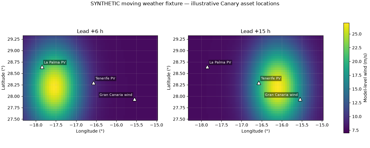
Asset-to-cell mapping:
             asset  face  x  y  latitude  longitude  distance_km  requested_latitude  requested_longitude
      Tenerife PV     0 16 35     28.30     -16.55        1.958               28.30               -16.57
Gran Canaria wind     0  9 55     27.95     -15.55        1.112               27.94               -15.55
      La Palma PV     0 23  9     28.65     -17.85        0.000               28.65               -17.85
3. Extract 24 hours and construct valid timestamps#
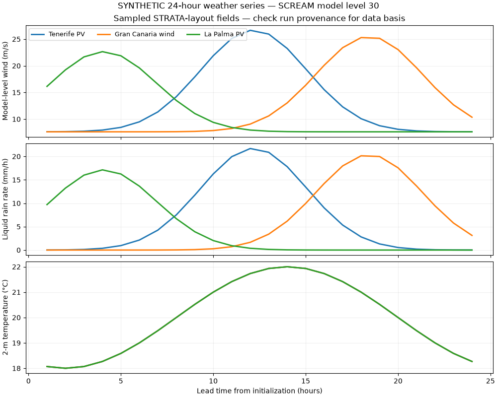
Each asset now has 24 valid-time rows. The first saved frame is +1 hour, not initialization. The reader loads the selected site fields, not the global weather cube. Output duration is derived from the saved leads. An hourly saved precipitation rate is an endpoint sample, not a one-hour accumulation; sparse output can miss short-lived precipitation peaks.
print("\nFirst asset, first three leads:\n", weather.head(3).round(3).to_string(index=False))
fig = plot_weather(weather)
fig.suptitle("SYNTHETIC 24-hour weather series — SCREAM model level 30")
plt.show()
First asset, first three leads:
       asset  lead_hours          valid_time  temperature_c  precipitation_mm_h  eastward_wind_ms  northward_wind_ms  interval_hours  wind_speed_ms  wind_model_level
Tenerife PV         1.0 2020-10-13 01:00:00         18.068               0.011             7.009              3.004             1.0          7.625                30
Tenerife PV         2.0 2020-10-13 02:00:00         18.000               0.040             7.033              3.013             1.0          7.651                30
Tenerife PV         3.0 2020-10-13 03:00:00         18.068               0.131             7.107              3.042             1.0          7.730                30
4. Demonstrate exact-pair forecast evaluation#
Real STRATA v1 predictions should be scored against SCREAM simulation output on held-out initializations. Calendar-matched AEMET/ERA5 weather is not truth for this historical simulation. This artificial reference has known offsets solely to test the evaluation plumbing. Its scores cannot establish STRATA skill. Persistence repeats the first saved forecast value; it is NOT a reference- initialization persistence forecast. No fitting or tuning uses this reference.
reference = weather.copy()
reference["wind_speed_ms"] -= 1.2
reference["precipitation_mm_h"] *= 0.85
reference["temperature_c"] -= 0.6
metrics = compare_reference(weather, reference)
print("\nSynthetic reference metrics (not model skill):\n", metrics.round(3).to_string(index=False))
Synthetic reference metrics (not model skill):
             asset           variable                  model  n   mae  rmse   bias
Gran Canaria wind      wind_speed_ms          STRATA output 24 1.200 1.200  1.200
Gran Canaria wind      wind_speed_ms First-lead persistence 24 5.090 7.516 -4.072
Gran Canaria wind precipitation_mm_h          STRATA output 24 0.901 1.406  0.901
Gran Canaria wind precipitation_mm_h First-lead persistence 24 5.106 7.968 -5.106
Gran Canaria wind      temperature_c          STRATA output 24 0.600 0.600  0.600
Gran Canaria wind      temperature_c First-lead persistence 24 1.568 1.943 -1.332
      La Palma PV      wind_speed_ms          STRATA output 24 1.200 1.200  1.200
      La Palma PV      wind_speed_ms First-lead persistence 24 7.215 7.888  5.686
      La Palma PV precipitation_mm_h          STRATA output 24 0.689 1.161  0.689
      La Palma PV precipitation_mm_h First-lead persistence 24 7.159 7.854  5.801
      La Palma PV      temperature_c          STRATA output 24 0.600 0.600  0.600
      La Palma PV      temperature_c First-lead persistence 24 1.568 1.943 -1.332
      Tenerife PV      wind_speed_ms          STRATA output 24 1.200 1.200  1.200
      Tenerife PV      wind_speed_ms First-lead persistence 24 5.355 8.049 -4.512
      Tenerife PV precipitation_mm_h          STRATA output 24 0.978 1.501  0.978
      Tenerife PV precipitation_mm_h First-lead persistence 24 5.531 8.500 -5.530
      Tenerife PV      temperature_c          STRATA output 24 0.600 0.600  0.600
      Tenerife PV      temperature_c First-lead persistence 24 1.568 1.943 -1.332
5. Translate exposure into an explicit business scenario#
The power plan is a separate, synthetic input: a daylight-shaped plan for PV and constant 45% capacity for wind. STRATA U/V do not become a hub-height turbine power curve, and T_2m/rain do not supply PV irradiance.
For demonstration, reduce interval power by 15% when wind >=20 m/s and 5% when rain >=15 mm/h; simultaneous alerts give a 20% reduction. These are analyst assumptions, not calibrated fragility or shutdown thresholds. E = baseline_MW * interval_hours * multiplier; gross value at risk is the energy difference * 60 EUR/MWh. This excludes tariffs, penalties and costs.
baseline = demo_baseline(weather, assets)
scenario = energy_scenario(weather, baseline, wind_threshold_ms=20, price_eur_mwh=60)
summary = scenario_summary(scenario)
print("\nHYPOTHETICAL energy scenario:\n", summary.round(3).to_string(index=False))

# Sensitivity scenarios are deterministic alternatives, not probabilities or
# confidence intervals. A threshold that changes the decision needs calibration.
thresholds = [16, 20, 24, 28]
sensitivity = [
    scenario_summary(energy_scenario(weather, baseline, wind_threshold_ms=value))
    for value in thresholds
]
fig, axes = plt.subplots(1, 2, figsize=(12, 4.8), layout="constrained")
axes[0].bar(summary.asset, summary.baseline_mwh, label="Baseline", color="#8bbcd0")
axes[0].bar(summary.asset, summary.scenario_mwh, label="Scenario", color="#185b78")
axes[0].set(ylabel="Energy (MWh)", title="Assumed production reductions")
axes[0].tick_params(axis="x", rotation=15)
axes[0].legend()
for asset in summary.asset:
    values = [
        float(row.loc[row.asset == asset, "energy_at_risk_mwh"].iloc[0]) for row in sensitivity
    ]
    axes[1].plot(thresholds, values, marker="o", label=asset)
axes[1].set(
    xlabel="Assumed model-level wind threshold (m/s)",
    ylabel="Energy at risk (MWh)",
    title="Threshold sensitivity; rain threshold fixed at 15 mm/h",
)
axes[1].legend(fontsize=8)
axes[1].grid(alpha=0.2)
fig.suptitle("SYNTHETIC energy scenarios — no predicted outage or financial return")
plt.show()
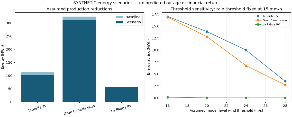
HYPOTHETICAL energy scenario:
             asset  baseline_mwh  scenario_mwh  energy_at_risk_mwh  gross_value_at_risk_eur  wind_alert_hours  rain_alert_hours
      Tenerife PV       114.919       101.047              13.872                   832.32               5.0               5.0
Gran Canaria wind       324.000       311.175              12.825                   769.50               5.0               4.0
      La Palma PV        57.460        57.460               0.000                     0.00               3.0               3.0
6. Reproduce and export the study#
Run from the repository root after installing the workspace:
uv run python -m energy_analysis.strata --demo --output artifacts/strata-demo
Outputs: weather.csv, asset_cells.csv, scenario.csv, summary.csv, weather.png and manifest.json (assumptions, software versions and CSV hashes). To export the artificial metrics shown above as well, use the Python API:
from pathlib import Path
from energy_analysis.strata import write_results
write_results(Path("artifacts/strata-gallery"), weather, cells,
              provenance={"data_basis": "SYNTHETIC gallery exercise"},
              scenario=scenario, metrics=metrics)
For real output, use the guide’s GPU workflow, then:
uv run --with 'zarr>=3,<4' python -m energy_analysis.strata \
  --input /path/to/strata_24h.zarr --assets assets.csv \
  --wind-level 30 --output artifacts/strata-real
Real mode exports weather only unless you supply an explicit –baseline CSV. Add –reference only for independently prepared, matching SCREAM truth. Keep successful upstream rollout logs: preallocated/unwritten Zarr chunks can appear as valid zero values, which finite-value checks alone cannot detect.
Decision boundary#
Use these results to inspect data coverage, test pipeline assumptions and identify measurements needed for a calibrated study. Operational curtailment, maintenance dispatch or revenue commitments require validated wind heights, asset response models, complete forecasts and appropriate forecast verification. STRATA itself is documented at NVlabs/STRATA.
Total running time of the script: (0 minutes 0.583 seconds)