Note
Go to the end to download the full example code.
UK low-wind electricity margin notice: conditional battery relief#
On 8 November 2026, Britain’s NESO issued an Electricity Margin Notice for 9 November. The Guardian reported an initial forecast reserve-margin shortfall of almost 1,400 MW for 06:00-11:00, an approximately 800 MW request for extra generation, and a later forecast margin shortfall of approximately 500 MW after market action. These figures are snapshots, not an observed hourly deficit series or lost electricity supply.
Source: https://www.theguardian.com/business/2026/nov/09/rare-call-more-electricity-supplies-windpower-drops-britain-energy-shortfall Operator winter outlook: https://www.neso.energy/british-electricity-supplies-secure-winter-despite-global-instability-1
Business question: under an explicitly HYPOTHETICAL constant-margin-gap stress case, how much precharged BESS power and usable DC energy would be needed to support the capacity margin for several hours? No UK outage, blackout risk or actual BESS dispatch is inferred from this screening plot.
import matplotlib.pyplot as plt

from energy_methods.margin_relief import screen_margin_relief

# News: separately reported forecast snapshots. The durations below come
# from reported notice windows, but the *constant deficit in every interval*
# is an explicitly SYNTHETIC stress scenario, NOT NESO telemetry.
scenarios = {
    "Initial notice (06-11, hypothetical constant 1400 MW)": (1400.0, 10),
    "Revised notice (08-11, hypothetical constant 500 MW)": (500.0, 6),
}
timestep_hours = 0.5
eta = 0.95  # ASSUMED illustrative discharge efficiency, not observed.
power_options = [500.0, 1000.0, 1500.0]  # HYPOTHETICAL MW power ratings.
stored_gwh = [0, 0.5, 1, 2, 4, 8, 10]  # HYPOTHETICAL precharged usable DC energy.
fig, axes = plt.subplots(1, 2, figsize=(13, 4.6), layout="constrained")
for ax, (label, (gap_mw, intervals)) in zip(axes, scenarios.items(), strict=True):
    gap_profile_mw = [gap_mw] * intervals  # SYNTHETIC interval profile.
    baseline = screen_margin_relief(
        gap_profile_mw,
        battery_power_mw=0,
        available_dc_energy_mwh=0,
        timestep_hours=timestep_hours,
        discharge_efficiency=eta,
    )
    for battery_mw in power_options:
        coverage = []
        for energy_gwh in stored_gwh:
            result = screen_margin_relief(
                gap_profile_mw,
                battery_power_mw=battery_mw,
                available_dc_energy_mwh=energy_gwh * 1000,
                timestep_hours=timestep_hours,
                discharge_efficiency=eta,
            )
            coverage.append(result.coverage_fraction * 100)
        ax.plot(stored_gwh, coverage, marker="o", label=f"{battery_mw / 1000:g} GW BESS")
    print(
        f"{label}: scenario margin-support equivalent "
        f"{baseline.margin_gap_mwh_equivalent / 1000:.2f} GWh, "
        f"no-storage coverage {baseline.coverage_fraction:.0%}; "
        f"minimum theoretical initial DC energy at >= {gap_mw:.0f} MW "
        f"= {baseline.margin_gap_mwh_equivalent / eta / 1000:.2f} GWh."
    )
    ax.set(
        xlabel="Initial usable DC energy above minimum SOC (GWh) — ASSUMED",
        ylabel="Hypothetical margin-gap coverage (%)",
        title=f"{gap_mw / 1000:g} GW for {intervals * timestep_hours:g} h (SYNTHETIC)",
        ylim=(0, 104),
    )
    ax.axhline(100, color="black", linestyle="--", linewidth=1)
    ax.legend()
plt.show()
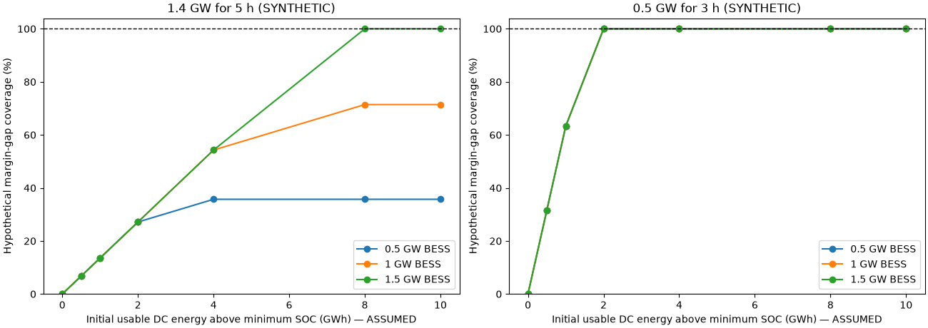
Initial notice (06-11, hypothetical constant 1400 MW): scenario margin-support equivalent 7.00 GWh, no-storage coverage 0%; minimum theoretical initial DC energy at >= 1400 MW = 7.37 GWh.
Revised notice (08-11, hypothetical constant 500 MW): scenario margin-support equivalent 1.50 GWh, no-storage coverage 0%; minimum theoretical initial DC energy at >= 500 MW = 1.58 GWh.
Interpret these as conditional power/energy capacity sensitivities ONLY. This is NOT demand left unserved, a historical margin time series, a reliability probability, or a forecast UK battery investment recommendation. Additional market actions and unmodeled grid and system-operability limits may dominate. Offline reproduction: uv run –no-sync python examples/analysis/plot_uk_low_wind_margin_2026.py
Total running time of the script: (0 minutes 0.148 seconds)