Note
Go to the end to download the full example code.
Worldwide climate degradation rates#
Recompute the combined rate and its three mechanisms from the saved 2016-2018 ERA5 study. These are modelled scenario rates in %/year, using published mono-Si coefficients and explicit stress-processing assumptions. They are not measured fleet degradation or a high-resolution reproduction of the thesis.
The grid samples land centres at 15° spacing. Of 71 sampled land locations, 63 have complete inputs across all three years; eight stay missing. Colored rectangles are coarse sample footprints, not uniform conditions across them.
Download the runnable bundle or
source and calibration provenance.
The guide explains regeneration,
attribution, regional mapping and scientific limits. This example runs offline.
import json
from pathlib import Path

import matplotlib.pyplot as plt
import numpy as np

from energy_analysis.degradation.gallery import load_degradation_example, plot_degradation_maps
from energy_methods.degradation import DegradationParameters
from energy_methods.degradation_mapping import map_degradation
Recompute from annual stresses#
The loader checks input hashes and recalculates every rate using the reusable methods package. It then checks the result against the original archived run. Temperature is module temperature; RH is percent; UV is the annual 280-400 nm dose. Missing inputs are never replaced with zero.
annual, rates, metadata = load_degradation_example(Path("."))
print(metadata["description"])
print(f"Valid land samples: {metadata['valid_cells']}/{metadata['land_cells']}")
print(f"Retrieved hourly location records: {metadata['hours_retrieved']:,}")
print(rates[["total_rate", "valid_year_count", "rate_class"]])
fig = plot_degradation_maps(rates, Path("climate_world_boundaries.geojson"))
plt.show()
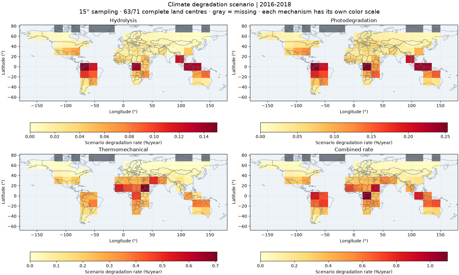
Real ERA5-derived annual stresses, 2016-2018; explicit mono-Si scenario
Valid land samples: 63/71
Retrieved hourly location records: 1,867,584
<xarray.Dataset> Size: 3kB
Dimensions:           (lat: 10, lon: 24)
Coordinates:
  * lat               (lat) float64 80B -60.0 -45.0 -30.0 ... 45.0 60.0 75.0
  * lon               (lon) float64 192B -172.5 -157.5 -142.5 ... 157.5 172.5
Data variables:
    total_rate        (lat, lon) float64 2kB nan nan nan nan ... nan nan nan nan
    valid_year_count  (lat, lon) int32 960B 0 0 0 0 0 0 0 0 ... 0 0 0 0 0 0 0 0
    rate_class        (lat, lon) int8 240B 0 0 0 0 0 0 0 0 0 ... 0 0 0 0 0 0 0 0
Attributes: (12/13)
    method:                  Kaaya climate degradation; thesis Eqs. 3.14-3.17...
    reference_ids:           ascencio_vasquez_2021_thesis ascencio_vasquez_20...
    baseline_start_year:     2016
    baseline_end_year:       2018
    aggregation:             mean_stress
    coverage_policy:         all stresses in every year
    ...                      ...
    source:                  Open-Meteo ERA5; normalized endpoint means; GHI-...
    calibration:             {"a_h": 49100000.0, "a_n": 1.0, "a_p": 71.83, "a...
    scope:                   Module-specific climate indicators; excludes LID...
    study_name:              Global degradation screening, 2016-2018 (15-degr...
    grid_step_degrees:       15.0
    spatial_interpretation:  nearest ERA5 sample at each CRU-supported centre...
Read rate categories without hiding missing cells#
The thesis mapping uses 0.2%/year bands. The combined expression is multiplicative: mechanism rates are not additive shares of the total. A number of 0.5 means 0.5%/year under this calibration, not 50%/year.
fig = plot_degradation_maps(rates, Path("climate_world_boundaries.geojson"), categorical=True)
plt.show()
print(
    f"Combined scenario range: {float(rates.total_rate.min()):.3f} to "
    f"{float(rates.total_rate.max()):.3f}%/year"
)
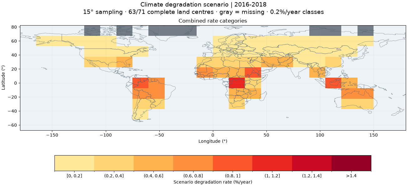
Combined scenario range: 0.019 to 1.101%/year
Check an aggregation choice#
Evaluating the model at mean stresses differs from averaging annual rates. This sensitivity calculation makes that choice visible. It is not a statistical uncertainty interval and does not address uncertainty in the module calibration.
parameters = DegradationParameters(**json.loads(Path("degradation_parameters.json").read_text()))
annual_rate_average = map_degradation(annual, parameters, aggregation="mean_rate")
difference = annual_rate_average.total_rate - rates.total_rate
print("Maximum absolute aggregation difference (%/year):", float(np.abs(difference).max()))
Maximum absolute aggregation difference (%/year): 0.002166271863138447
What to do with the map#
Use it to screen climate-driven mechanisms and choose locations for more detailed studies. For a project, retrieve local hourly weather, specify mounting and module calibration, and compare the model with measured performance loss. Do not turn the coarse global sample nearest a site into a site degradation forecast or use this scenario directly as a warranty or lifetime estimate. The guide gives NetCDF/GeoJSON export commands and a regional-study workflow.
Total running time of the script: (0 minutes 1.049 seconds)