Note
Go to the end to download the full example code.
Native satellite imagery with Orbital PV#
Read real, attributed crops through Orbital PV’s checksum-verified loader. The Tenerife example demonstrates 10 m Sentinel-2 site context, calibrated red reflectance and the separate 20 m scene classification. The Altadena example demonstrates sub-metre WorldView imagery from a disaster-response open archive. It does not identify a PV installation or assess damage at that location.
The highest-detail selection is scoped to this area, event and date range. No interpolation, sharpening or overview read creates finer native detail. The coloured display product and panchromatic analytical band are distinct.
Install Python 3.13, this package and the pinned Orbital PV integration; see the
satellite imagery guide.
Download the complete example and native crops.
All execution here is offline; the explicit live capture script is
scripts/prepare_satellite_imagery_samples.py.
Credits: Orbital PV, Element 84 Earth Search and Copernicus Sentinel data (2026). WorldView samples © Maxar/Vantor, CC BY-NC 4.0; cropped without resampling. The imagery licence is separate from the repository’s code licence.
import json
from dataclasses import asdict
from pathlib import Path

import matplotlib.pyplot as plt
import numpy as np
from matplotlib.colors import BoundaryNorm, ListedColormap

from energy_data_retrieval.sources.orbitalpv_imagery import (
    describe_asset,
    load_satellite_image,
)

DATA = (
    Path(globals().get("__file__", Path.cwd() / "plot_satellite_imagery.py")).resolve().parent
    / "data"
)
manifest = json.loads((DATA / "imagery_provenance.json").read_text())
images = {
    row["fixture"]: load_satellite_image(str(DATA / row["fixture"])) for row in manifest["samples"]
}


def draw(ax, image, values, title, **kwargs):
    """Display native pixel centres in projected metres, without smoothing."""
    left, bottom, right, top = image.bounds
    extent = (0, right - left, 0, top - bottom)
    artist = ax.imshow(values, extent=extent, origin="upper", interpolation="nearest", **kwargs)
    ax.set(title=title, xlabel="East from crop edge (m)", ylabel="North from crop edge (m)")
    ax.set_facecolor("#e9edf1")
    return artist


def rgb(image):
    values = np.moveaxis(image.data.filled(0), 0, -1).astype(float) / 255
    alpha = (~np.ma.getmaskarray(image.data).any(axis=0)).astype(float)
    return np.dstack((values, alpha))
Site context, reflectance and local scene quality#
A low scene-wide cloud percentage does not guarantee a cloud-free site. Inspect the SCL layer at its native 20 m spacing. The red reflectance uses the provider’s explicit scale and offset; RGB display bytes are not reflectance.
visual = images["imagery_tenerife_visual.tif"]
red = images["imagery_tenerife_red.tif"]
scl = images["imagery_tenerife_scl.tif"]
fig_sentinel, axes = plt.subplots(1, 3, figsize=(14, 5.4), layout="constrained")
draw(axes[0], visual, rgb(visual), "Sentinel-2 RGB · 10 m")
artist = draw(
    axes[1],
    red,
    red.reflectance()[0],
    "Surface red reflectance · 10 m",
    cmap="magma",
    vmin=0,
    vmax=0.4,
)
fig_sentinel.colorbar(artist, ax=axes[1], shrink=0.75, label="Unitless reflectance")
scl_colors = [
    "#000000",
    "#ff0000",
    "#444444",
    "#885522",
    "#228833",
    "#ddbb66",
    "#2266dd",
    "#999999",
    "#bbbbbb",
    "#ffffff",
    "#66ccff",
    "#ff99cc",
]
artist = draw(
    axes[2],
    scl,
    scl.data[0],
    "Scene classification · 20 m",
    cmap=ListedColormap(scl_colors),
    norm=BoundaryNorm(np.arange(-0.5, 12.5), 12),
)
fig_sentinel.colorbar(artist, ax=axes[2], shrink=0.75, ticks=range(12), label="Native SCL class")
fig_sentinel.suptitle("Icor area, Tenerife · Sentinel-2 site context", fontsize=17, weight="bold")
fig_sentinel.text(
    0.02,
    -0.035,
    (
        "Contains modified Copernicus Sentinel data (2026), processed by ESA; "
        "Earth Search distribution. Native pixels, no cloud masking."
    ),
    fontsize=9,
)
print("Sentinel scene:", visual.scene_id)
print("Red band resolution and metadata:", asdict(describe_asset(red.item_metadata, "red")))
print(
    "SCL class counts:",
    dict(zip(*np.unique(scl.data.compressed(), return_counts=True), strict=True)),
)
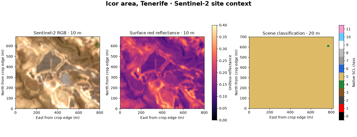
Sentinel scene: S2A_T28RCS_20260804T115232_L2A
Red band resolution and metadata: {'scene_id': 'S2A_T28RCS_20260804T115232_L2A', 'asset_key': 'red', 'product_kind': 'spectral', 'native_gsd_m': 10.0, 'grid_spacing_m': (10.0, 10.0), 'detail_limit_m': 10.0, 'acquisition_utc': '2026-08-04T11:53:59.065000Z', 'platform': 'sentinel-2a'}
SCL class counts: {np.uint8(4): np.int64(1), np.uint8(5): np.int64(1434)}
Sub-metre satellite imagery: native detail versus display spacing#
The panchromatic image has one broad spectral band. A percentile stretch below changes screen contrast only; the saved uint16 values stay untouched. The RGB image is the provider’s 8-bit pansharpened display product. Its finer output grid is not an improvement in the sensor’s native sampling.
pan = images["imagery_altadena_pan_analytic.tif"]
colour = images["imagery_altadena_visual.tif"]
pan_info = describe_asset(pan.item_metadata, "pan_analytic")
colour_info = describe_asset(colour.item_metadata, "visual")
low, high = np.percentile(pan.data.compressed(), [2, 98])
fig_worldview, axes = plt.subplots(1, 2, figsize=(11, 6.5), layout="constrained")
draw(
    axes[0],
    pan,
    pan.data[0],
    (
        f"Panchromatic · declared GSD {pan_info.native_gsd_m:.2f} m\n"
        f"Native raster spacing {pan.transform[0]:.3f} m"
    ),
    cmap="gray",
    vmin=low,
    vmax=high,
)
draw(
    axes[1],
    colour,
    rgb(colour),
    (
        f"Provider pansharpened RGB\nDisplay grid {colour.transform[0]:.3f} m; "
        f"detail bound {colour_info.detail_limit_m:.2f} m"
    ),
)
fig_worldview.suptitle("Altadena · WorldView-3 · 8 January 2025", fontsize=17, weight="bold")
fig_worldview.text(
    0.02,
    -0.025,
    (
        "© Maxar/Vantor Open Data Program · CC BY-NC 4.0 · Event-limited coverage. "
        "Native crops; pan contrast stretched for display only."
    ),
    fontsize=9,
)
print("WorldView scene:", pan.scene_id)
print("Acquisition and licence provenance:", pan.item_metadata["properties"]["edi:open_data"])
print("Panchromatic resolution:", asdict(pan_info))
print("RGB display resolution:", asdict(colour_info))
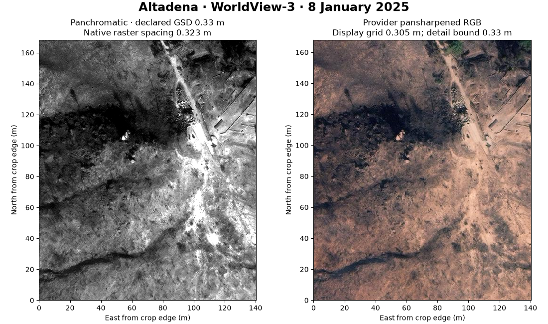
WorldView scene: 11/031311103031/104001009C64B300
Acquisition and licence provenance: {'event': 'WildFires-LosAngeles-Jan-2025', 'event_url': 'https://maxar-opendata.s3.amazonaws.com/events/WildFires-LosAngeles-Jan-2025/collection.json', 'event_license': 'CC-BY-NC-4.0', 'acquisition_license': 'proprietary', 'item_url': 'https://maxar-opendata.s3.amazonaws.com/events/WildFires-LosAngeles-Jan-2025/ard/11/031311103031/2025-01-08/104001009C64B300.json'}
Panchromatic resolution: {'scene_id': '11/031311103031/104001009C64B300', 'asset_key': 'pan_analytic', 'product_kind': 'panchromatic', 'native_gsd_m': 0.33, 'grid_spacing_m': (0.32330209347614414, 0.32330209347614414), 'detail_limit_m': 0.33, 'acquisition_utc': '2025-01-08 18:41:38Z', 'platform': 'WV03'}
RGB display resolution: {'scene_id': '11/031311103031/104001009C64B300', 'asset_key': 'visual', 'product_kind': 'rendered_pansharpened_rgb', 'native_gsd_m': 0.33, 'grid_spacing_m': (0.30517578125, 0.30517578125), 'detail_limit_m': 0.33, 'acquisition_utc': '2025-01-08 18:41:38Z', 'platform': 'WV03'}
What to do with the result#
Retain the TIFF and its .meta.json together. Use native georeferencing for
overlays with surveyed PV footprints and the terrain connector; reproject
explicitly when combining different grids. Inspect nodata, clouds, shadows,
capture dates and positional uncertainty before tracing site features.
Fine imagery supports visual interpretation of roofs, roads and array rows
where visible. It does not by itself establish installed capacity, measured
generation or degradation. Use PVGIS for resource/modelled yield and dated
meter observations for performance; keep image-derived hypotheses separate.
plt.show()
Total running time of the script: (0 minutes 0.665 seconds)