Note
Go to the end to download the full example code.
PVGIS 5: all seven data endpoints for one site#
Retrieve modelled solar resource and PV estimates for a coordinate in Tenerife (28.4775° N, 16.3294° W). These complete real API captures are unmodified and include native input/output metadata and retrieval provenance. No plant measurements are implied. The gallery runs offline.
Download the complete runnable bundle and read
the endpoint guide for both API versions.
from pathlib import Path

import matplotlib.pyplot as plt
import pandas as pd

from energy_data_retrieval.sources.pvgis import load_response
1. Make explicit requests in your own workflow#
These are the seven calls used to acquire the saved responses. They are shown here, rather than executed during a documentation build:
from energy_data_retrieval.transport import HTTPClient
from energy_data_retrieval.sources.pvgis import PVGISClient, PVGIS_HOSTS
with HTTPClient(PVGIS_HOSTS) as http:
    api = PVGISClient(http)  # explicit /api/v5_3; version="5.2" also supported
    pv = api.grid_connected(28.4775, -16.3294, peakpower=1, loss=14, angle=25)
    monthly = api.monthly_radiation(28.4775, -16.3294, horirrad=True,
                                    avtemp=True, startyear=2020, endyear=2020)
    daily = api.daily_radiation(28.4775, -16.3294, month=6, **{"global": True})
    offgrid = api.off_grid(28.4775, -16.3294, peakpower=1000,
                          batterysize=2000, consumptionday=3000, cutoff=20)
    horizon = api.horizon(28.4775, -16.3294)
    hourly = api.hourly(28.4775, -16.3294, startyear=2020, endyear=2020,
                       components=True, pvcalculation=True, peakpower=1, loss=14)
    tmy = api.typical_year(28.4775, -16.3294)
    pv.save(Path("my_pv.json"))  # response plus .provenance.json
Grid-connected peak power is kW; off-grid peak power is W, battery
capacity is Wh, and daily demand is Wh/day. No automatic unit conversion
takes place in the connector. Native aspect is south=0°, west=90°.
2. Verify all seven captures and retain their metadata#
folder = Path(globals().get("__file__", Path.cwd() / "plot_pvgis_legacy.py")).resolve().parent
responses = {
    name: load_response(folder / "data" / f"pvgis_v5_{name}.json")
    for name in ("pv", "monthly", "daily", "offgrid", "horizon", "hourly", "tmy")
}
for name, response in responses.items():
    print(name, response.request.retrieved_at_utc, response.request.sha256)
print("PV input metadata:", responses["pv"].json()["inputs"])
print("PV output definitions:", responses["pv"].json()["meta"]["outputs"])

pv = responses["pv"].table("outputs", "monthly", "fixed")
monthly = responses["monthly"].table("outputs", "monthly")
daily = responses["daily"].table("outputs", "daily_profile")
offgrid = responses["offgrid"].table("outputs", "monthly")
hourly = responses["hourly"].table("outputs", "hourly")
horizon = responses["horizon"].table("outputs", "horizon_profile")
pv 2026-10-31T07:39:07.638576+00:00 ef140ee26018fcca2feb17bb3fdbec7bcb6f5edd813843d2f0ee6100d4ea0b0f
monthly 2026-10-31T07:39:11.374845+00:00 b33602cc092da74593fb389d13f17ce39bb0a9b0dd328d58539437717b956a70
daily 2026-10-31T07:39:15.009153+00:00 744446a2bdb075ad47f66f8309fbe46ac8f19043eb407c7d67a04e7d7674f421
offgrid 2026-10-31T07:39:18.713308+00:00 9a14e66a56b35114be92d86892ce52198e965520ffa7275890674f8bd26a8768
horizon 2026-10-31T07:39:22.292554+00:00 b4917b9a53ed532c945b1638071617ce0070b81dc37e912202e0410448844cd5
hourly 2026-10-31T07:39:27.998684+00:00 7858013c1a4723946cb701974d31c3b3ce39fd03d36c0ab522389757125d3a64
tmy 2026-10-31T07:39:33.194958+00:00 ad0e03d4ce765e206a58c59adaaa57520b1c6e3f24330347c7b79f8a6412c5ab
PV input metadata: {'location': {'latitude': 28.4775, 'longitude': -16.3294, 'elevation': 622.0}, 'meteo_data': {'radiation_db': 'PVGIS-SARAH3', 'meteo_db': 'ERA5', 'year_min': 2005, 'year_max': 2023, 'use_horizon': True, 'horizon_db': 'DEM-calculated'}, 'mounting_system': {'fixed': {'slope': {'value': 25, 'optimal': False}, 'azimuth': {'value': 0, 'optimal': False}, 'type': 'free-standing'}}, 'pv_module': {'technology': 'c-Si', 'peak_power': 1.0, 'system_loss': 14.0}, 'economic_data': {'system_cost': None, 'interest': None, 'lifetime': None}}
PV output definitions: {'monthly': {'type': 'time series', 'timestamp': 'monthly averages', 'variables': {'E_d': {'description': 'Average daily energy production from the given system', 'units': 'kWh/d'}, 'E_m': {'description': 'Average monthly energy production from the given system', 'units': 'kWh/mo'}, 'H(i)_d': {'description': 'Average daily sum of global irradiation per square meter received by the modules of the given system', 'units': 'kWh/m2/d'}, 'H(i)_m': {'description': 'Average monthly sum of global irradiation per square meter received by the modules of the given system', 'units': 'kWh/m2/mo'}, 'SD_m': {'description': 'Standard deviation of the monthly energy production due to year-to-year variation', 'units': 'kWh'}}}, 'totals': {'type': 'time series totals', 'variables': {'E_d': {'description': 'Average daily energy production from the given system', 'units': 'kWh/d'}, 'E_m': {'description': 'Average monthly energy production from the given system', 'units': 'kWh/mo'}, 'E_y': {'description': 'Average annual energy production from the given system', 'units': 'kWh/y'}, 'H(i)_d': {'description': 'Average daily sum of global irradiation per square meter received by the modules of the given system', 'units': 'kWh/m2/d'}, 'H(i)_m': {'description': 'Average monthly sum of global irradiation per square meter received by the modules of the given system', 'units': 'kWh/m2/mo'}, 'H(i)_y': {'description': 'Average annual sum of global irradiation per square meter received by the modules of the given system', 'units': 'kWh/m2/y'}, 'SD_m': {'description': 'Standard deviation of the monthly energy production due to year-to-year variation', 'units': 'kWh'}, 'SD_y': {'description': 'Standard deviation of the annual energy production due to year-to-year variation', 'units': 'kWh'}, 'l_aoi': {'description': 'Angle of incidence loss', 'units': '%'}, 'l_spec': {'description': 'Spectral loss', 'units': '%'}, 'l_tg': {'description': 'Temperature and irradiance loss', 'units': '%'}, 'l_total': {'description': 'Total loss', 'units': '%'}}}}
3. Different endpoints answer different questions#
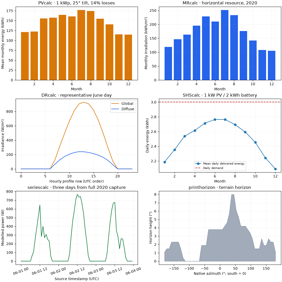
Each panel retains its own period and system settings. The hourly request uses the default horizontal plane; the PVcalc request uses 25° tilt. The daily irradiance is a representative June profile, not an observed calendar day.
fig, axes = plt.subplots(3, 2, figsize=(11, 11), layout="constrained")
ax = axes[0, 0]
ax.bar(pv["month"], pv["E_m"], color="#d97706")
ax.set(
    title="PVcalc · 1 kWp, 25° tilt, 14% losses", xlabel="Month", ylabel="Mean monthly energy (kWh)"
)
ax = axes[0, 1]
ax.bar(monthly["month"], monthly["H(h)_m"], color="#2563eb")
ax.set(
    title="MRcalc · horizontal resource, 2020",
    xlabel="Month",
    ylabel="Monthly irradiation (kWh/m²)",
)
ax = axes[1, 0]
ax.plot(range(len(daily)), daily["G(i)"], color="#d97706", label="Global")
ax.plot(range(len(daily)), daily["Gd(i)"], color="#2563eb", label="Diffuse")
ax.set(
    title="DRcalc · representative June day",
    xlabel="Hourly profile row (UTC order)",
    ylabel="Irradiance (W/m²)",
)
ax.legend()
ax = axes[1, 1]
ax.plot(offgrid["month"], offgrid["E_d"] / 1000, marker="o", label="Mean daily delivered energy")
ax.axhline(3, linestyle="--", color="#b91c1c", label="Daily demand")
ax.set(title="SHScalc · 1 kW PV / 2 kWh battery", xlabel="Month", ylabel="Daily energy (kWh)")
ax.legend(fontsize=8)
ax = axes[2, 0]
time = pd.to_datetime(hourly["time"], format="%Y%m%d:%H%M", utc=True)
selection = (time >= "2020-06-01") & (time < "2020-06-04")
ax.plot(time[selection], hourly.loc[selection, "P"], color="#15803d")
ax.set(
    title="seriescalc · three days from full 2020 capture",
    xlabel="Source timestamp (UTC)",
    ylabel="Modelled power (W)",
)
ax.tick_params(axis="x", rotation=20)
ax = axes[2, 1]
ax.fill_between(horizon["A"], horizon["H_hor"], color="#64748b", alpha=0.6)
ax.set(
    title="printhorizon · terrain horizon",
    xlabel="Native azimuth (°; south = 0)",
    ylabel="Horizon height (°)",
)
for ax in axes.flat:
    ax.grid(alpha=0.15)
plt.show()
4. TMY is a composite year with explicit selected source months#
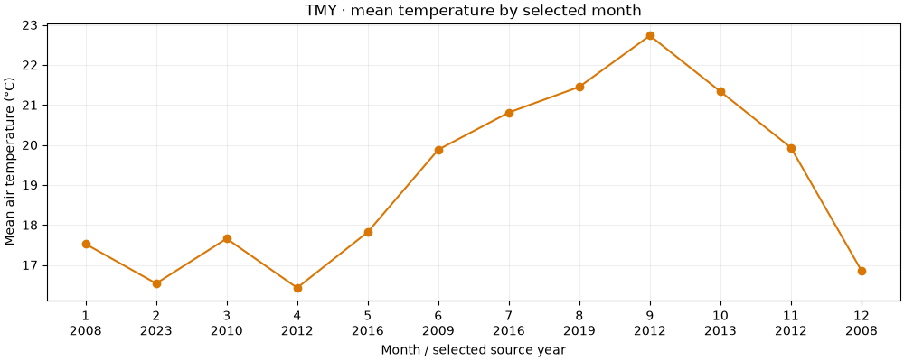
Keep the provider’s selected years. Do not sort the timestamps into a claimed continuous historical year. This plot groups the complete 8,760-hour TMY by month number and displays the selected source year below each month.
tmy = responses["tmy"].table("outputs", "tmy_hourly")
selected = responses["tmy"].table("outputs", "months_selected")
print(selected.to_string(index=False))
print("TMY input metadata:", responses["tmy"].json()["inputs"])
month = pd.to_datetime(tmy["time(UTC)"], format="%Y%m%d:%H%M").dt.month
means = tmy.groupby(month)["T2m"].mean()
fig, ax = plt.subplots(figsize=(10, 4), layout="constrained")
ax.plot(means.index, means.values, marker="o", color="#d97706")
ax.set_xticks(
    selected["month"],
    [f"{m}\n{y}" for m, y in zip(selected["month"], selected["year"], strict=True)],
)
ax.set(
    title="TMY · mean temperature by selected month",
    xlabel="Month / selected source year",
    ylabel="Mean air temperature (°C)",
)
ax.grid(alpha=0.2)
plt.show()
 month  year
     1  2008
     2  2023
     3  2010
     4  2012
     5  2016
     6  2009
     7  2016
     8  2019
     9  2012
    10  2013
    11  2012
    12  2008
TMY input metadata: {'location': {'latitude': 28.4775, 'longitude': -16.3294, 'elevation': 622.0, 'irradiance_time_offset': 0.1526}, 'meteo_data': {'radiation_db': 'PVGIS-SARAH3', 'meteo_db': 'ERA5', 'year_min': 2005, 'year_max': 2023, 'use_horizon': True, 'horizon_db': 'DEM-calculated'}}
What to do with these data#
Use monthly resource and PVcalc for screening, hourly data for a reproducible
PV/yield workflow, TMY for a typical-year building or system simulation, and
SHScalc to screen off-grid demand/battery combinations. The off-grid result
here does not satisfy the whole stated demand; inspect f_e and E_miss
before selecting a battery. Horizon data can identify terrain obstruction but
do not establish vegetation or building shading at the real array.
Metadata retains the selected database, source period, model settings and
field units. Reanalysis/satellite estimates are not onsite sensors. The
:09 hourly timestamp offset is retained; no rounding or timezone guess is
made by the connector. Model calibration and site evidence remain separate.
print("Off-grid totals:", responses["offgrid"].json()["outputs"]["totals"])
Off-grid totals: {'d_total': 6939.0, 'f_f': 83.14, 'f_e': 99.99, 'E_lost': 1612.34, 'E_miss': 498.43}
Total running time of the script: (0 minutes 0.551 seconds)