Note
Go to the end to download the full example code.
Reliability algorithms: lifetime, failure causes, redundancy and repairs#
Synthetic device histories demonstrate usable algorithms. These are not raw observations reconstructed from the published PV papers. Historical component rates and real-source evidence have their own connector and analysis examples.
Existing Poisson, Gamma-Poisson, Beta-binomial and censored Weibull methods are combined with paired bootstrap bounds, Aalen-Johansen competing risks, an independent k-out-of-n model, and a two-state repairable availability model.
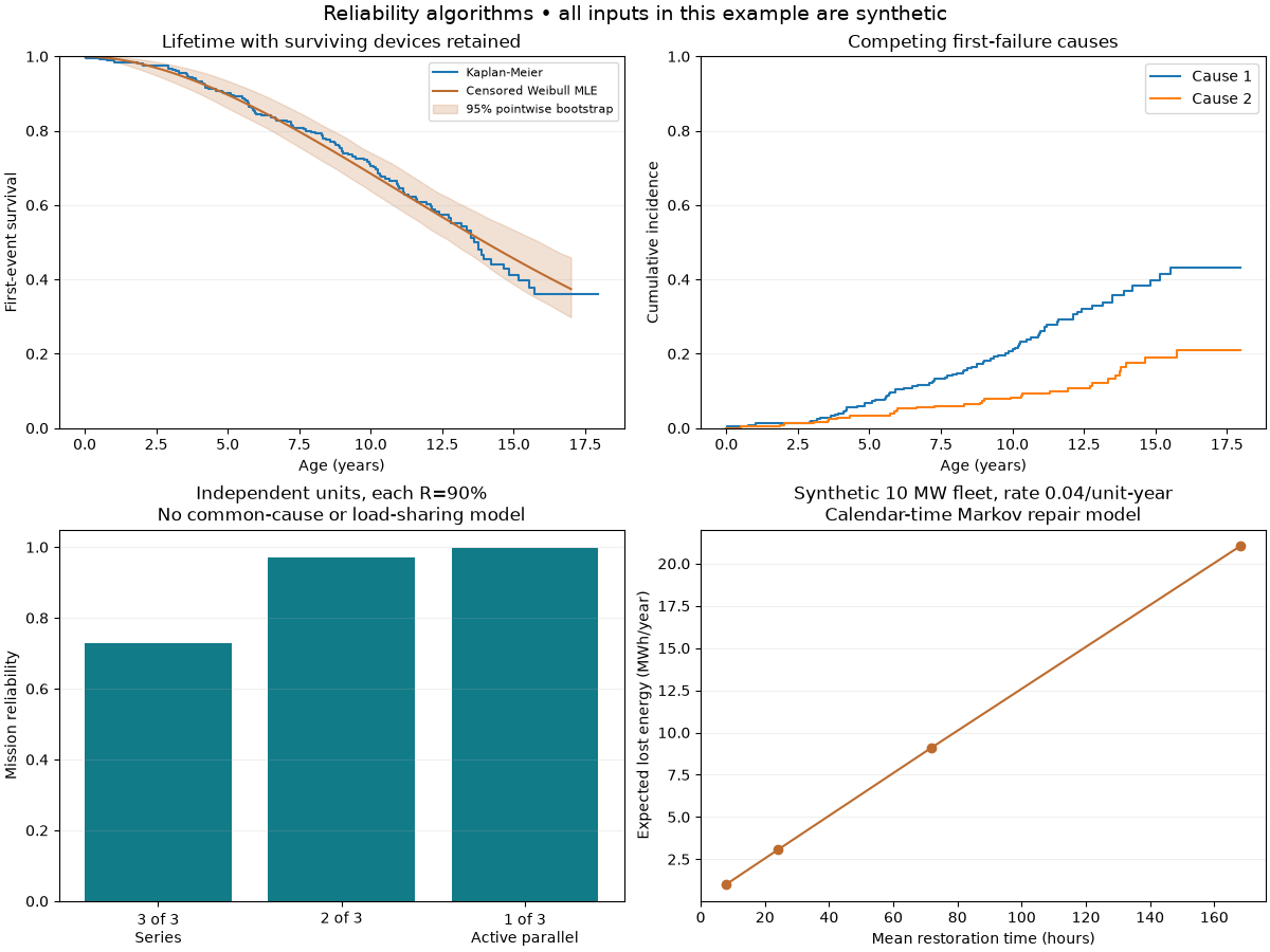
Synthetic events/unit-year and exact 95% interval: RateEstimate(failures=12, exposure=300, rate=0.04, lower=0.02066858369574073, upper=0.06987195016058986, confidence=0.95)
Synthetic posterior mean and 95% interval: 0.04 (0.021868372218001714, 0.06351541690902535)
Predictive P(at least one event in 100 unit-years): 0.97035322700137
Synthetic stow-demand failure probability and interval: 0.005 (0.001034034897982096, 0.012008761418637558)
Synthetic Weibull shape, scale (years): 1.7956016568932163 17.16053116971008
Synthetic P(failure next year | survived to 10): 0.06833425995076636
Synthetic restoration / energy sensitivity:
  mean_restore_hours  assumed_rate_per_unit_year  mean_availability  baseline_energy_mwh  expected_energy_loss_mwh         input_kind
                  8                        0.04           0.999964         27963.736151                  1.020775 synthetic_scenario
                 24                        0.04           0.999891         27963.736151                  3.056080 synthetic_scenario
                 72                        0.04           0.999674         27963.736151                  9.115320 synthetic_scenario
                168                        0.04           0.999248         27963.736151                 21.024718 synthetic_scenario
import matplotlib.pyplot as plt
import numpy as np

from energy_analysis.pv_device_reliability import repair_time_sensitivity
from energy_methods.failure_rates import BetaDemand, GammaRate, estimate_rate, fit_weibull_censored
from energy_methods.pv_device_reliability import kaplan_meier_survival
from energy_methods.reliability_algorithms import (
    aalen_johansen,
    bootstrap_weibull_survival,
    k_out_of_n_reliability,
)

# Synthetic fleet: 12 verified events / 300 summed unit-years. The prior is an
# explicitly assumed Gamma with shape=2, rate=50 unit-years, not a paper fit.
rate = estimate_rate(12, 300)
posterior = GammaRate(2, 50).update(12, 300)
print("Synthetic events/unit-year and exact 95% interval:", rate)
print("Synthetic posterior mean and 95% interval:", posterior.mean, posterior.interval())
print(
    "Predictive P(at least one event in 100 unit-years):", posterior.probability_at_least_one(100)
)
stow = BetaDemand(1, 99).update(2, 500)  # Assumed prior + synthetic demands.
print("Synthetic stow-demand failure probability and interval:", stow.mean, stow.interval())

rng = np.random.default_rng(5)
lifetime = 15 * rng.weibull(2.2, 250)
follow_up = rng.uniform(8, 18, 250)
ages = np.minimum(lifetime, follow_up)
failed = lifetime <= follow_up
km = kaplan_meier_survival(ages, failed)
weibull = fit_weibull_censored(ages, failed)
curve = bootstrap_weibull_survival(ages, failed, np.linspace(0, 17, 90), resamples=200)
print("Synthetic Weibull shape, scale (years):", weibull.parameter1, weibull.parameter2)
print("Synthetic P(failure next year | survived to 10):", weibull.conditional_failure(10, 1))

# Mutually exclusive first-failure causes; survivors remain code 0.
causes = np.where(failed, rng.choice([1, 2], size=ages.size, p=[0.65, 0.35]), 0)
incidence = aalen_johansen(ages, causes)
repair = repair_time_sensitivity()
print("Synthetic restoration / energy sensitivity:\n", repair.to_string(index=False))

fig, axes = plt.subplots(2, 2, figsize=(12, 9), layout="constrained")
fig.suptitle("Reliability algorithms • all inputs in this example are synthetic", fontsize=14)
ax = axes[0, 0]
ax.step(np.r_[0, km.age], np.r_[1, km.survival], where="post", label="Kaplan-Meier")
ax.plot(curve.age, curve.survival, color="#bd6b2e", label="Censored Weibull MLE")
ax.fill_between(
    curve.age, curve.lower, curve.upper, color="#bd6b2e", alpha=0.2, label="95% pointwise bootstrap"
)
ax.set(
    xlabel="Age (years)",
    ylabel="First-event survival",
    ylim=(0, 1),
    title="Lifetime with surviving devices retained",
)
ax.legend(fontsize=8)

ax = axes[0, 1]
for column, label in [("incidence_1", "Cause 1"), ("incidence_2", "Cause 2")]:
    ax.step(np.r_[0, incidence.age], np.r_[0, incidence[column]], where="post", label=label)
ax.set(
    xlabel="Age (years)",
    ylabel="Cumulative incidence",
    ylim=(0, 1),
    title="Competing first-failure causes",
)
ax.legend()

ax = axes[1, 0]
ax.bar(
    ["3 of 3\nSeries", "2 of 3", "1 of 3\nActive parallel"],
    [k_out_of_n_reliability([0.9, 0.9, 0.9], k) for k in [3, 2, 1]],
    color="#117b88",
)
ax.set(
    ylabel="Mission reliability",
    ylim=(0, 1.05),
    title="Independent units, each R=90%\nNo common-cause or load-sharing model",
)

ax = axes[1, 1]
ax.plot(repair.mean_restore_hours, repair.expected_energy_loss_mwh, "o-", color="#bd6b2e")
ax.set(
    xlabel="Mean restoration time (hours)",
    ylabel="Expected lost energy (MWh/year)",
    title="Synthetic 10 MW fleet, rate 0.04/unit-year\nCalendar-time Markov repair model",
)
for ax in axes.flat:
    ax.grid(axis="y", alpha=0.2)
plt.show()
Total running time of the script: (0 minutes 0.603 seconds)